In my previous post I looked the latest release of Oracle Stream Analytics (OSA), and saw how it provided a graphical interface to “Fast Data”. Users can analyse streaming data as it arrives based on conditions and rules. They can also transform the stream data, publishing it back out as a stream in its own right. In this article we’ll see how OSA can be used with Kafka.

Kafka is one of the foremost streaming technologies nowadays, for very good reasons. It is highly scalable and flexible, supporting multiple concurrent consumers. Oracle Streaming Analytics supports Kafka as both a source and target. To set up an inbound stream from Kafka, first we define the Connection:

Once the Connection is defined, we can create a Stream for a given Kafka topic:

If you get an error at this point of Unable to deploy OEP application then check the OSA log – it could be a connectivity issue to Zookeeper.

Exception in thread "SpringOsgiExtenderThread-286" org.springframework.beans.FatalBeanException:
Error in context lifecycle initialization; nested exception is com.bea.wlevs.ede.api.EventProcessingException: 
org.I0Itec.zkclient.exception.ZkTimeoutException: 
Unable to connect to zookeeper server within timeout: 6000

Assuming that the Stream is saved with no errors, you can then create an Exploration based on the stream and all being well, the live tweets are soon shown. Unlike the example at the top of this article, these tweets are coming in via Kafka, rather than the built-in OSA Twitter Stream. This is partly to demonstrate the Kafka capabilities, but also because the built-in OSA Twitter Stream only includes a subset of the available twitter data fields.

Avro? Nope.

Data in Kafka can be serialised in many formats, including Avro – which OSA doesn’t seem to like. No error is thrown to the GUI but the exploration remains blank.

Looking in the OSA log file there’s a whole lot of errors recorded similar to this:

line 1:0 no viable alternative at character '?'
line 1:1 no viable alternative at character '?'
line 1:2 no viable alternative at character '?'
line 1:3 no viable alternative at character '?'
line 1:4 no viable alternative at character '?'
line 1:5 no viable alternative at character '?'
line 1:6 no viable alternative at character '?'
line 1:7 no viable alternative at character '?'
line 1:8 no viable alternative at character ''

JSON? Kinda.

One of the challenges that I found working with OSA was defining the “Shape” (data model) of the inbound stream data. JSON is a format used widely as a technology-agnostic data interchange format, including for the twitter data that I was working with. You can see a sample record here. One of the powerful features of JSON is its ability to nest objects in a record, as well as create arrays of them. You can read more about this detail in a recent article I wrote here. Unfortunately it seems that OSA does not support flattening out JSON, meaning that only elements in the root of the model are accessible. For twitter, that means we can see the text, and who it was in reply to, but not the user who tweeted it, since the latter is a nested element (along with many other fields, including hashtags which are also an array):

root
|-- created_at: string (nullable = true)
|-- entities: struct (nullable = true)
|    |-- hashtags: array (nullable = true)
|    |    |-- element: struct (containsNull = true)
|    |    |    |-- indices: array (nullable = true)
|    |    |    |    |-- element: long (containsNull = true)
|    |    |    |-- text: string (nullable = true)
|    |-- user_mentions: array (nullable = true)
|    |    |-- element: struct (containsNull = true)
|    |    |    |-- id: long (nullable = true)
|    |    |    |-- id_str: string (nullable = true)
|    |    |    |-- indices: array (nullable = true)
|    |    |    |    |-- element: long (containsNull = true)
|    |    |    |-- name: string (nullable = true)
|    |    |    |-- screen_name: string (nullable = true)
|-- source: string (nullable = true)
|-- text: string (nullable = true)
|-- timestamp_ms: string (nullable = true)
|-- truncated: boolean (nullable = true)
|-- user: struct (nullable = true)
|    |-- followers_count: long (nullable = true)
|    |-- following: string (nullable = true)
|    |-- friends_count: long (nullable = true)
|    |-- name: string (nullable = true)
|    |-- screen_name: string (nullable = true)

So what to do if the inbound streaming data is in nested-JSON format? It seems to me the only option is to pre-process it to flatten it. There are a variety of tools that could be used here – in the first instance I’d generally reach for Logstash, it being the one I’m most familiar with. To get an idea of the schema of a JSON record you can use jsonschema.net. Funnily enough when I was researching this blog post I came across the exact same problem on a forum posted by … me! Early last year I was working with the same dataset, and had the same issue with embedded arrays. The way to do it in Logstash is with a bit of Ruby code to flatten the arrays, and a standard mutate to bring nested objects up to the root level. Sample code:

mutate {  
    add_field => { "user_name" => "%{[user][name]}" }  
    add_field => { "user_screen_name" => "%{[user][screen_name]}" }  
}
ruby {  
    code => 'event["hashtags_array"] = event["[entities][hashtags]"].collect { |m| m["text"] } unless event["[entities][hashtags]"].nil?  
             event["hashtags_list"] = event["hashtags_array"].join(",")  unless event["[hashtags_array]"].nil?'  
}

You can find the full Logstash code on gist here. With this logstash code running I set up a new OSA Stream pointing to the new Kafka topic that Logstash was writing, and added the flattened fields to the Shape:

We can then see in the Exploration the fields that we wanted to get at – user name, hashtags, and so on:

Other Shape Gotchas

One of the fields in Twitter data is ‘source’ – which unfortunately is a reserved identifier in the CQL language that OSA uses behind the scenes.

Caused By: org.springframework.beans.FatalBeanException: Exception initializing channel; nested exception is com.bea.wlevs.ede.api.ConfigurationException: Event type [sx-10-16-Kafka_Technology_Tweets_JSON-1] of channel [channel] uses invalid or reserved CQL identifier = , source

It’s not clear how to define a shape in which the source data field is named after a reserved identifier.

Further Exploration of Twitter Streams with OSA

Using the flattened Twitter stream coming via Kafka that I demonstrated above, let’s now look at more OSA functionality.

Depending on the source of your data stream, and your purpose for analysing it, you may well want to filter out certain content. This can be done from the Exploration screen:

The Business Rules section of the Exploration enables you to define rules about the data and set field values based on it. This can be static values, or expressions based on data in the stream. There doens’t seem to be a way to add arbitrary fields via this, so I amended the Stream Shape to include a ‘spare’ field that I then populated:

Kafka Stream Transformation with OSA

Here we’ll see how OSA can be used to ingest one Kafka topic, apply a transformation, and stream it to another Kafka topic.

The OSA exploration screen offers a basic aggregation (‘summary’) function, here showing the number of tweets per language:

Using the Windows icon to the right of the Sources box the time window can be defined, along with the refresh frequency:

This means that the count of tweets per language will be calculated looking at the data for the past 30 seconds, and this will be evaluated every five seconds. More complex functionality such as pivoting on the group-by column (so as to be able to chart out the number of tweets per language as separate metrics) doesn’t seem to be present in this release; arguably this is moving over into per analytics territory such as would be found in Oracle’s Big Data Discovery.

Taking the summarised stream (count of tweets, by language) I first Publish the exploration, making it available for use as the input to a subsequent exploration. Then from the Catalog page select a Pattern, which I’m going to use to build a stream showing the most common languages in the past five seconds. With the Top N pattern you specify the event stream (in this case, the summarised stream that I built above), and the metric by which to order the events which here is the count of tweets per language.

For completeness, I’m going to stream the output of this pattern exploration back to a Kafka topic

Note that I’ve defined a new Shape here based on the columns in the pattern. In the pattern itself I renamed the COUNT column to a clearer one (tweet_count_5_sec). Renaming it wasn’t strictly necessary since it’s possible to define the field/shape mapping when you configure the Target:

For the target to take effect, I publish the pattern exploration, and then using kafka-console-consumer can see the topic being populated in realtime by OSA:

Being able to apply transformations to streams in realtime like this and stream the results is pretty useful. There are some limitations to the capabilities of OSA through the front end GUI. For example, support for nested json, and integration with the Kafka Schema Registry to automatically derive Shapes for inbound topics would both be great. Lower-level, the option to specify the consumer group id, as well as the start point for consumption (beginning of topic, or streaming at the end) are both things that would probably be necessary sooner or later using OSA for full-blown development.

OSA and Spatial

One of the Patterns that OSA provides is a Spatial one, which can be used to analyse source data that includes geo-location data. This could be to simply plot the occurrence of the data point (as we’ll see shortly) on a map. It can also be used in a more sophisticated manner, to track a given entity’s movements on a map. An example of this could be a fleet of trucks reporting their position back at regular intervals. Areas on a map can be defined and conditions triggered as the entity enters or leaves the area. For now though, we’ll keep it simple. Using the flattened Twitter stream from Kafka that I produced from Logstash above, I’m going to plot Tweets in realtime on a map, along with a very simplistic tagging of the broad area in which they came from.

In my source Kafka topic I have two fields, latitude and longitude. I expose these as part of the ‘flattening’ of the JSON in this logstash script, since by default they’re nested within the coordinates field and as an array too. When defining the Stream’s Shape make sure you define the datatype correctly (Double) – OSA is not very forgiving of stupidity and I spent a frustrating time trying to work out why “-80.1422195” was coming through as zero – obviously defined as an Integer this was never going to work!

Not entirely necessary, but useful for debug purposes, I setup an exploration based on the flattened Twitter stream, with a filter to only include tweets that had geo-location data in them. This way I knew what tweets I should expect to be seeing in the next step. One of the things that I have found with OSA is that it has a tendency to fail silently; instead of throwing errors you’ll just not get any data. By setting up the filter exploration I could at least debug things a bit more easily.

After this I created a new object, a Map. A Map object defines a set of named areas, which could be sourced from a database table, or drawn manually – which is what I did here by setting the Map Type to ‘None (Create Manually)’. One thing to note about the maps is that they’re sourced online (openstreetmap.org) so you’ll need an internet connection to do this. Once the Map is open, click the Polygon Tool icon and click-drag a shape around the area that you want to “geo-fence”. Each area is given a name, and this is what is used in the streaming data to label the event’s geographical area.

Having got our source data stream with geo-data in, and a Map on which to plot it and analyse the location of each event, we now use the Spatial General pattern to create an Exploration. The topology looks like this:

The fields in the Spatial General pattern are all pretty obvious. Object key is the field to use to track the same entity across multiple events, if you want to use the enter/exit/stay statuses. For tweets we just use ‘Enter’, but for people or vehicles, for example, you might get multiple status reports and want to track them on a map. For example, when a person is near a point of interest that you’re tracking, or a vehicle has remained in a set area for too long.

If you let the Exploration now run, depending on the rate of event ingest, you’ll sooner or later see points appearing on the map and event details underneath. The “status” column is populated (blank if the event is outside of the defined geo-fences), as is the “Place”, based on the geo-fence names that you defined.

Summary

I can see OSA being used in two ways. The first as an ‘endpoint’ for streams with users taking actions based on the data, with some of the use cases listed here. The second is for prototyping transformations and analyses on streams prior to productionising them. The visual interface and immediacy of feedback on transformations applied means that users can quickly understand what further processing they may want to apply to the stream using actual streaming data to inform this.

This latter concept – that of prototyping – is similar to that which we see with another of Oracle’s products, Big Data Discovery. With BDD users can analyse data in the organisation’s data reservoir, as well as apply transformations to it (read more). Just as BDD doesn’t replace OBIEE or Visual Analyzer but enables users to understand how they do want to model the data in these tools, OSA wouldn’t replace “production grade” integration done by Oracle Data Integrator. What it would do is allow users to get a clearer idea of the transformations they would want performed in it.

OSA’s user interface is easy to use and intuitive, and this is definitely a tool that you would put in front of technically minded business users. There are limitations to what can be achieved technically through the web GUI alone and something like Oracle Data Integrator (ODI) would still be a more appropriate fit for complex streaming work. At Oracle Open World last year it was announced (slides) that a beta would be starting for ODI using Spark Streaming for ETL and stream processing, so it’ll be interesting to see this when it comes out.

Further Reading

• Providing Oracle Stream Analytics 12c environment using Docker, by Guido Schmutz
• Real-Time Data Streaming & Exploration with Oracle GoldenGate & Oracle Stream Analytics, by Issam Hijazi
• Demonstration of Oracle Stream Explorer for live device monitoring – collect, filter, aggregate, pattern match, enrich and publish by Lucas Jellema
• OTN OSA home page
• Documentation index
  • Use cases
  • Installation

The post Stream Analytics and Processing with Kafka and Oracle Stream Analytics appeared first on Rittman Mead Consulting.

Big Data Discovery (BDD) is a great tool for exploring, transforming, and visualising data stored in your organisation’s Data Reservoir. I presented a workshop on it at a recent conference, and got an interesting question from the audience that I thought I’d explore further here. Currently the primary route for getting data into BDD requires that it be (i) in HDFS and (ii) have a Hive table defined on top of it. From there, BDD automagically ingests the Hive table, or the dataprocessingCLI is manually called which prompts the BDD DGraph engine to go and sample (or read in full) the Hive dataset.

This is great, and works well where the dataset is vast (this is Big Data, after all) and needs the sampling that DGraph provides. It’s also simple enough for Hive tables that have already been defined, perhaps by another team. But - and this was the gist of the question that I got - what about where the Hive table doesn’t exist already? Because if it doesn’t, we now need to declare all the columns as well as choose the all-important SerDe in order to read the data.

SerDes are brilliant, in that they enable the application of a schema-on-read to data in many forms, but at the very early stages of a data project there are probably going to be lots of formats of data (such as TSV, CSV, JSON, as well as log files and so on) from varying sources. Choosing the relevant SerDe for each one, and making sure that BDD is also configured with the necessary jar, as well as manually listing each column to be defined in the table, adds overhead to the project. Wouldn’t it be nice if we could side-step this step somehow? In this article we’ll see how!

Importing Datasets through BDD Studio

Before we get into more fancy options, don’t forget that BDD itself offers the facility to upload CSV, TSV, and XLSX files, as well as connect to JDBC datasources. Data imported this way will be stored by BDD in a Hive table and ingested to DGraph.

This is great for smaller files held locally. But what about files on your BDD cluster, that are too large to upload from local machine, or in other formats - such as JSON?

Loading a CSV file

As we’ve just seen, CSV files can be imported to Hive/BDD directly through the GUI. But perhaps you’ve got a large CSV file sat local to BDD that you want to import? Or a folder full of varying CSV files that would be too time-consuming to upload through the GUI one-by-one?

For this we can use BDD Shell with the Python Pandas library, and I’m going to do so here through the excellent Jupyter Notebooks interface. You can read more about these here and details of how to configure them on BigDataLite 4.5 here. The great thing about notebooks, whether Jupyter or Zeppelin, is that I don’t need to write any more blog text here - I can simply embed the notebook inline and it is self-documenting:

https://gist.github.com/76b477f69303dd8a9d8ee460a341c445

(gist link)

Note that at end of this we call dataprocessingCLI to automatically bring the new table into BDD’s DGraph engine for use in BDD Studio. If you’ve got BDD configured to automagically add new Hive tables, or you don’t want to run this step, you can just comment it out.

Loading simple JSON data

Whilst CSV files are tabular by definition, JSON records can contain nested objects (recursively), as well as arrays. Let’s look at an example of using SparkSQL to import a simple flat JSON file, before then considering how we handle nested and array formats. Note that SparkSQL can read datasets from both local (file://) storage as well as HDFS (hdfs://):

https://gist.github.com/8b7118c230f34f7d57bd9b0aa4e0c34c

(gist link)

Once loaded into Hive, it can be viewed in Hue:

Loading nested JSON data

What’s been great so far, whether loading CSV, XLS, or simple JSON, is that we’ve not had to list out column names. All that needs modifying in the scripts above to import a different file with a different set of columns is to change the filename and the target tablename. Now we’re going to look at an example of a JSON file with nested objects - which is very common in JSON - and we’re going to have to roll our sleeves up a tad and start hardcoding some schema details.

First up, we import the JSON to a SparkSQL dataframe as before (although this time I’m loading it from HDFS, but local works too):

df = sqlContext.read.json('hdfs:///user/oracle/incoming/twitter/2016/07/12/')  

Then I declare this as a temporary table, which enables me to subsequently run queries with SQL against it

df.registerTempTable("twitter")  

A very simple example of a SQL query would be to look at the record count:

result_df = sqlContext.sql("select count(*) from twitter")  
result_df.show()

+----+  
| _c0|  
+----+  
|3011|  
+----+

The result of a sqlContext.sql invocation is a dataframe, which above I’m assigning to a new variable, but I could as easily run:

sqlContext.sql("select count(*) from twitter").show()  

for the same result.

The sqlContext has inferred the JSON schema automagically, and we can inspect it using

df.printSchema()  

The twitter schema is huge, so I’m just quoting a few choice sections of it here to illustrate subsequent points:

root  
|-- created_at: string (nullable = true)  
|-- entities: struct (nullable = true)  
|    |-- hashtags: array (nullable = true)  
|    |    |-- element: struct (containsNull = true)  
|    |    |    |-- indices: array (nullable = true)  
|    |    |    |    |-- element: long (containsNull = true)  
|    |    |    |-- text: string (nullable = true)  
|    |-- user_mentions: array (nullable = true)  
|    |    |-- element: struct (containsNull = true)  
|    |    |    |-- id: long (nullable = true)  
|    |    |    |-- id_str: string (nullable = true)  
|    |    |    |-- indices: array (nullable = true)  
|    |    |    |    |-- element: long (containsNull = true)  
|    |    |    |-- name: string (nullable = true)  
|    |    |    |-- screen_name: string (nullable = true)  
|-- source: string (nullable = true)  
|-- text: string (nullable = true)  
|-- timestamp_ms: string (nullable = true)  
|-- truncated: boolean (nullable = true)  
|-- user: struct (nullable = true)  
|    |-- followers_count: long (nullable = true)  
|    |-- following: string (nullable = true)  
|    |-- friends_count: long (nullable = true)  
|    |-- name: string (nullable = true)  
|    |-- screen_name: string (nullable = true)

Points to note about the schema:

• In the root of the schema we have attributes such as text and created_at
• There are nested elements (“struct”) such as user and within it screen_name, followers_count etc
• There’s also array objects, where an attribute can occur more than one, such as hashtags, and user_mentions.

Accessing root and nested attributes is easy - we just use dot notation:

sqlContext.sql("SELECT created_at, user.screen_name, text FROM twitter").show()

+--------------------+--------------+--------------------+  
|          created_at|   screen_name|                text|  
+--------------------+--------------+--------------------+  
|Tue Jul 12 16:13:...|  Snehalstocks|"Students need to...|  
|Tue Jul 12 16:13:...|   KingMarkT93|Ga caya :( https:...|

We can save this as a dataframe that’s then persisted to Hive, for ingest into BDD:

subset02 = sqlContext.sql("SELECT created_at, user.screen_name, text FROM twitter")  
tablename = 'twitter_user_text'  
qualified_tablename='default.' + tablename  
subset02.write.mode('Overwrite').saveAsTable(qualified_tablename)  

Which in Hue looks like this:

Attributes in an array are a bit more tricky. Here’s an example tweet with multiple user_mentions and a hashtag too:

https://twitter.com/flederbine/status/752940179569115136

Here we use the LATERAL VIEW syntax, with the optional OUTER operator since not all tweets have these additional entities, and we want to make sure we show all tweets including those that don’t have these entities. Here’s the SQL formatted for reading:

SELECT id,  
created_at,  
user.screen_name,  
text as tweet_text,  
hashtag.text as hashtag,  
user_mentions.screen_name as mentioned_user  
from twitter  
LATERAL VIEW OUTER explode(entities.user_mentions) user_mentionsTable as user_mentions  
LATERAL VIEW OUTER explode(entities.hashtags) hashtagsTable AS hashtag  

Which when run as from sqlContext.sql() gives us:

+------------------+--------------------+---------------+--------------------+-------+---------------+  
|                id|          created_at|    screen_name|          tweet_text|hashtag|    screen_name|  
+------------------+--------------------+---------------+--------------------+-------+---------------+  
|752940179569115136|Tue Jul 12 18:58:...|     flederbine|@johnnyq72 @orcld...|ImALLin|      johnnyq72|  
|752940179569115136|Tue Jul 12 18:58:...|     flederbine|@johnnyq72 @orcld...|ImALLin|       orcldoug|  
|752940179569115136|Tue Jul 12 18:58:...|     flederbine|@johnnyq72 @orcld...|ImALLin|          rmoff|  
|752940179569115136|Tue Jul 12 18:58:...|     flederbine|@johnnyq72 @orcld...|ImALLin|    markrittman|  
|752940179569115136|Tue Jul 12 18:58:...|     flederbine|@johnnyq72 @orcld...|ImALLin|     mikedurran|  
+------------------+--------------------+---------------+--------------------+-------+---------------+

and written back to Hive for ingest to BDD:

You can use these SQL queries both for simply flattening JSON, as above, or for building summary tables, such as this one showing the most common hashtags in the dataset:

sqlContext.sql("SELECT hashtag.text,count(*) as inst_count from twitter  LATERAL VIEW OUTER explode(entities.hashtags) hashtagsTable AS hashtag GROUP BY hashtag.text order by inst_count desc").show(4)

+-----------+----------+  
|       text|inst_count|  
+-----------+----------+  
|     Hadoop|       165|  
|     Oracle|       151|  
|        job|       128|  
|    BigData|       112|

You can find the full Jupyter Notebook with all these nested/array JSON examples here:

https://gist.github.com/a38e853d3a7dcb48a9df99ce1e3505ff

(gist link)

You may decide after looking at this that you’d rather just go back to Hive and SerDes, and as is frequently the case in ‘data wrangling’ there’s multiple ways to achieve the same end. The route you take comes down to personal preference and familiarity with the toolsets. In this particular case I'd still go for SparkSQL for the initial exploration as it's quicker to 'poke around' the dataset than with defining and re-defining Hive tables -- YMMV. A final point to consider before we dig in is that SparkSQL importing JSON and saving back to HDFS/Hive is a static process, and if your underlying data is changing (e.g. streaming to HDFS from Flume) then you would probably want a Hive table over the HDFS file so that it is live when queried.

Loading an Excel workbook with many sheets

This was the use-case that led me to researching programmatic import of datasets in the first place. I was doing some work with a dataset of road traffic accident data, which included a single XLS file with over 30 sheets, each a lookup table for a separate set of dimension attributes. Importing each sheet one by one through the BDD GUI was tedious, and being a lazy geek, I looked to automate it.

Using Pandas read_excel function and a smidge of Python to loop through each sheet it was easily done. You can see the full notebook here:

https://gist.github.com/rmoff/3fa5d857df8ca5895356c22e420f3b22

(gist link)

Oracle's Big Data Discovery encompasses a good amount of exploration, transformation, and visualisation capabilities for datasets residing in your organisation’s data reservoir. Even with this though, there may come a time when your data scientists want to unleash their R magic on those same datasets. Perhaps the data domain expert has used BDD to enrich and cleanse the data, and now it's ready for some statistical analysis? Maybe you'd like to use R's excellent forecast package to predict the next six months of a KPI from the BDD dataset? And not only predict it, but write it back into the dataset for subsequent use in BDD? This is possible using BDD Shell and rpy2. It enables advanced analysis and manipulation of datasets already in BDD. These modified datasets can then be pushed back into Hive and then BDD.

BDD Shell provides a native Python environment, and you may opt to use the pandas library to work with BDD datasets as detailed here. In other cases you may simply prefer working with R, or have a particular library in mind that only R offers natively. In this article we’ll see how to do that. The "secret sauce" is rpy2 which enables the native use of R code within a python-kernel Jupyter Notebook.

As with previous articles I’m using a Jupyter Notebook as my environment. I’ll walk through the code here, and finish with a copy of the notebook so you can see the full process.

First we'll see how you can use R in Jupyter Notebooks running a python kernel, and then expand out to integrate with BDD too. You can view and download the first notebook here.

Import the RPY2 environment so that we can call R from Jupyter

import readline is necessary to workaround the error: /u01/anaconda2/lib/libreadline.so.6: undefined symbol: PC

import readline

%load_ext rpy2.ipython

Example usage

%R X=c(1,4,5,7); sd(X); mean(X)

array([ 4.25])

%%R
Y = c(2,4,3,9)
summary(lm(Y~X))

Call:  
lm(formula = Y ~ X)

Residuals:  
    1     2     3     4  
 0.88 -0.24 -2.28  1.64 

Coefficients:  
            Estimate Std. Error t value Pr(>|t|)  
(Intercept)   0.0800     2.3000   0.035    0.975  
X             1.0400     0.4822   2.157    0.164

Residual standard error: 2.088 on 2 degrees of freedom  
Multiple R-squared:  0.6993,    Adjusted R-squared:  0.549  
F-statistic: 4.651 on 1 and 2 DF,  p-value: 0.1638

%R plot(X, Y)

import numpy as np
Z = np.array([1,4,5,10])

%R -i Z mean(Z)

array([ 5.])

Working with BDD Datasets from R in Jupyter Notebooks

execfile('ipython/00-bdd-shell-init.py')  
%load_ext rpy2.ipython

I also found that I had to make readline available otherwise I got an error (/u01/anaconda2/lib/libreadline.so.6: undefined symbol: PC)

import readline  

After this, we can import a BDD dataset, convert it to a Spark dataframe and then a pandas dataframe, ready for passing to R

ds = dss.dataset('edp_cli_edp_8d6fd230-8e99-449c-9480-0c2bddc4f6dc')  
spark_df = ds.to_spark()  
import pandas as pd  
pandas_df = spark_df.toPandas()  

Note that there is a lot of passing of the same dataframe into different memory structures here - from BDD dataset context to Spark to Pandas, and that’s before we’ve even hit R. It’s fine for ad-hoc wrangling but might start to be painful with very large datasets.

Now we use the rpy2 integration with Jupyter Notebooks and invoke R parsing of the cell’s contents, using the %%R syntax. Optionally, we can pass across variables with the -i parameter, which we’re doing here. Then we assign the dataframe to an R-notation variable (optional, but stylistically nice to do), and then use R's summary function to show a summary of each attribute:

%%R -i pandas_df  
R.df <- pandas_df  
summary(R.df)  

vendorid     tpep_pickup_datetime tpep_dropoff_datetime passenger_count  
 Min.   :1.000   Min.   :1.420e+12    Min.   :1.420e+12     Min.   :0.000  
 1st Qu.:1.000   1st Qu.:1.427e+12    1st Qu.:1.427e+12     1st Qu.:1.000  
 Median :2.000   Median :1.435e+12    Median :1.435e+12     Median :1.000  
 Mean   :1.525   Mean   :1.435e+12    Mean   :1.435e+12     Mean   :1.679  
 3rd Qu.:2.000   3rd Qu.:1.443e+12    3rd Qu.:1.443e+12     3rd Qu.:2.000  
 Max.   :2.000   Max.   :1.452e+12    Max.   :1.452e+12     Max.   :9.000  
 NA's   :12      NA's   :12           NA's   :12            NA's   :12     
 trip_distance      pickup_longitude  pickup_latitude    ratecodeid    
 Min.   :    0.00   Min.   :-121.93   Min.   :-58.43   Min.   : 1.000  
 1st Qu.:    1.00   1st Qu.: -73.99   1st Qu.: 40.74   1st Qu.: 1.000  
 Median :    1.71   Median : -73.98   Median : 40.75   Median : 1.000  
 Mean   :    3.04   Mean   : -72.80   Mean   : 40.10   Mean   : 1.041  
 3rd Qu.:    3.20   3rd Qu.: -73.97   3rd Qu.: 40.77   3rd Qu.: 1.000  
 Max.   :67468.40   Max.   : 133.82   Max.   : 62.77   Max.   :99.000  
 NA's   :12         NA's   :12        NA's   :12       NA's   :12      
 store_and_fwd_flag dropoff_longitude dropoff_latitude  payment_type 
 N   :992336        Min.   :-121.93   Min.   : 0.00    Min.   :1.00  
 None:    12        1st Qu.: -73.99   1st Qu.:40.73    1st Qu.:1.00  
 Y   :  8218        Median : -73.98   Median :40.75    Median :1.00  
                    Mean   : -72.85   Mean   :40.13    Mean   :1.38  
                    3rd Qu.: -73.96   3rd Qu.:40.77    3rd Qu.:2.00  
                    Max.   :   0.00   Max.   :44.56    Max.   :5.00  
                    NA's   :12        NA's   :12       NA's   :12    
  fare_amount          extra            mta_tax          tip_amount     
 Min.   :-170.00   Min.   :-1.0000   Min.   :-1.7000   Min.   :  0.000  
 1st Qu.:   6.50   1st Qu.: 0.0000   1st Qu.: 0.5000   1st Qu.:  0.000  
 Median :   9.50   Median : 0.0000   Median : 0.5000   Median :  1.160  
 Mean   :  12.89   Mean   : 0.3141   Mean   : 0.4977   Mean   :  1.699  
 3rd Qu.:  14.50   3rd Qu.: 0.5000   3rd Qu.: 0.5000   3rd Qu.:  2.300  
 Max.   : 750.00   Max.   :49.6000   Max.   :52.7500   Max.   :360.000  
 NA's   :12        NA's   :12        NA's   :12        NA's   :12       
  tolls_amount      improvement_surcharge  total_amount       PRIMARY_KEY     
 Min.   : -5.5400   Min.   :-0.3000       Min.   :-170.80   0-0-0   :      1  
 1st Qu.:  0.0000   1st Qu.: 0.3000       1st Qu.:   8.75   0-0-1   :      1  
 Median :  0.0000   Median : 0.3000       Median :  11.80   0-0-10  :      1  
 Mean   :  0.3072   Mean   : 0.2983       Mean   :  16.01   0-0-100 :      1  
 3rd Qu.:  0.0000   3rd Qu.: 0.3000       3rd Qu.:  17.80   0-0-1000:      1  
 Max.   :503.0500   Max.   : 0.3000       Max.   : 760.05   0-0-1001:      1  
 NA's   :12         NA's   :12            NA's   :12        (Other) :1000560  

We can use native R code and R libraries including the excellent dplyr to lightly wrangle and then chart the data:

%%R

library(dplyr)  
library(ggplot2)

R.df %>%  
    filter(fare_amount > 0) %>%  
    ggplot(aes(y=fare_amount, x=tip_amount,color=passenger_count)) +  
    geom_point(alpha=0.5 )

Finally, using the -o flag on the %%R invocation, we can pass back variables from the R context back to pandas :

%%R -o R_output  
R_output <-  
    R.df %>%  
    mutate(foo = 'bar')

and from there back to Spark and write the results to Hive:

spark_df2 = sqlContext.createDataFrame(R_output)  
spark_df2.write.mode('Overwrite').saveAsTable('default.updated_dataset')  

and finally ingest the new Hive table to BDD:

from subprocess import call  
call(["/u01/bdd/v1.2.0/BDD-1.2.0.31.813/dataprocessing/edp_cli/data_processing_CLI","--table default.updated_dataset"])  

You can download the notebook here.

https://gist.github.com/6f7d3138efdbb322d8543d35912c99ab

Oracle Stream Analytics (OSA) is a graphical tool that provides “Business Insight into Fast Data”. In layman terms, that translates into an intuitive web-based interface for exploring, analysing, and manipulating streaming data sources in realtime. These sources can include REST, JMS queues, as well as Kafka. The inclusion of Kafka opens OSA up to integration with many new-build data pipelines that use this as a backbone technology.

• Streams - definitions of sources of data such as Kafka, JMS, and a dummy data generator (event generator)
• Connections - Servers etc from which Streams are defined
• Explorations - front-end for seeing contents of Streams in realtime, as well as applying light transformations
• Targets - destination for transformed streams

Viewing Realtime Twitter Data with OSA

Adding Lookup Data to Streams

attr_id,attr_value  
1,never  
2,gonna  
3,give  
4,you  
5,up  

Daisy-Chaining, Targets, and Topology

Once an Exploration is Published it can be used as the Source for subsequent Explorations, enabling you to map out a pipeline based on multiple source streams and transformations. Here we're taking the exploration created just above that joined the two streams together, and using the output as the source for a new Exploration:

In the next post I will look at how Oracle Stream Analytics can be used to analyse, enrich, and publish data to and from Kafka. Stay tuned!

In my previous post I looked the latest release of Oracle Stream Analytics (OSA), and saw how it provided a graphical interface to "Fast Data". Users can analyse streaming data as it arrives based on conditions and rules. They can also transform the stream data, publishing it back out as a stream in its own right. In this article we'll see how OSA can be used with Kafka.

Kafka is one of the foremost streaming technologies nowadays, for very good reasons. It is highly scalable and flexible, supporting multiple concurrent consumers. Oracle Streaming Analytics supports Kafka as both a source and target. To set up an inbound stream from Kafka, first we define the Connection:

Exception in thread "SpringOsgiExtenderThread-286" org.springframework.beans.FatalBeanException:  
Error in context lifecycle initialization; nested exception is com.bea.wlevs.ede.api.EventProcessingException:  
org.I0Itec.zkclient.exception.ZkTimeoutException:  
Unable to connect to zookeeper server within timeout: 6000  

Avro? Nope.

Data in Kafka can be serialised in many formats, including Avro - which OSA doesn’t seem to like. No error is thrown to the GUI but the exploration remains blank.

  
line 1:0 no viable alternative at character '?'  
line 1:1 no viable alternative at character '?'  
line 1:2 no viable alternative at character '?'  
line 1:3 no viable alternative at character '?'  
line 1:4 no viable alternative at character '?'  
line 1:5 no viable alternative at character '?'  
line 1:6 no viable alternative at character '?'  
line 1:7 no viable alternative at character '?'  
line 1:8 no viable alternative at character ''  

JSON? Kinda.

root
|-- created_at: string (nullable = true)
|-- entities: struct (nullable = true)
|    |-- hashtags: array (nullable = true)
|    |    |-- element: struct (containsNull = true)
|    |    |    |-- indices: array (nullable = true)
|    |    |    |    |-- element: long (containsNull = true)
|    |    |    |-- text: string (nullable = true)
|    |-- user_mentions: array (nullable = true)
|    |    |-- element: struct (containsNull = true)
|    |    |    |-- id: long (nullable = true)
|    |    |    |-- id_str: string (nullable = true)
|    |    |    |-- indices: array (nullable = true)
|    |    |    |    |-- element: long (containsNull = true)
|    |    |    |-- name: string (nullable = true)
|    |    |    |-- screen_name: string (nullable = true)
|-- source: string (nullable = true)
|-- text: string (nullable = true)
|-- timestamp_ms: string (nullable = true)
|-- truncated: boolean (nullable = true)
|-- user: struct (nullable = true)
|    |-- followers_count: long (nullable = true)
|    |-- following: string (nullable = true)
|    |-- friends_count: long (nullable = true)
|    |-- name: string (nullable = true)
|    |-- screen_name: string (nullable = true)

mutate {  
    add_field => { "user_name" => "%{[user][name]}" }  
    add_field => { "user_screen_name" => "%{[user][screen_name]}" }  
}
ruby {  
    code => 'event["hashtags_array"] = event["[entities][hashtags]"].collect { |m| m["text"] } unless event["[entities][hashtags]"].nil?  
             event["hashtags_list"] = event["hashtags_array"].join(",")  unless event["[hashtags_array]"].nil?'  
}

Other Shape Gotchas

One of the fields in Twitter data is ‘source’ - which unfortunately is a reserved identifier in the CQL language that OSA uses behind the scenes.

Caused By: org.springframework.beans.FatalBeanException: Exception initializing channel; nested exception is com.bea.wlevs.ede.api.ConfigurationException: Event type [sx-10-16-Kafka_Technology_Tweets_JSON-1] of channel [channel] uses invalid or reserved CQL identifier = , source

It’s not clear how to define a shape in which the source data field is named after a reserved identifier.

Further Exploration of Twitter Streams with OSA

Using the flattened Twitter stream coming via Kafka that I demonstrated above, let’s now look at more OSA functionality.

Depending on the source of your data stream, and your purpose for analysing it, you may well want to filter out certain content. This can be done from the Exploration screen:

Kafka Stream Transformation with OSA

Here we’ll see how OSA can be used to ingest one Kafka topic, apply a transformation, and stream it to another Kafka topic.

The OSA exploration screen offers a basic aggregation (‘summary’) function, here showing the number of tweets per language:

Taking the summarised stream (count of tweets, by language) I first Publish the exploration, making it available for use as the input to a subsequent exploration. Then from the Catalog page select a Pattern, which I’m going to use to build a stream showing the most common languages in the past five seconds. With the Top N pattern you specify the event stream (in this case, the summarised stream that I built above), and the metric by which to order the events which here is the count of tweets per language.

Note that I’ve defined a new Shape here based on the columns in the pattern. In the pattern itself I renamed the COUNT column to a clearer one (tweetcount5_sec). Renaming it wasn’t strictly necessary since it’s possible to define the field/shape mapping when you configure the Target:

OSA and Spatial

One of the Patterns that OSA provides is a Spatial one, which can be used to analyse source data that includes geo-location data. This could be to simply plot the occurrence of the data point (as we'll see shortly) on a map. It can also be used in a more sophisticated manner, to track a given entity's movements on a map. An example of this could be a fleet of trucks reporting their position back at regular intervals. Areas on a map can be defined and conditions triggered as the entity enters or leaves the area. For now though, we'll keep it simple. Using the flattened Twitter stream from Kafka that I produced from Logstash above, I'm going to plot Tweets in realtime on a map, along with a very simplistic tagging of the broad area in which they came from.

In my source Kafka topic I have two fields, latitude and longitude. I expose these as part of the 'flattening' of the JSON in this logstash script, since by default they're nested within the coordinates field and as an array too. When defining the Stream's Shape make sure you define the datatype correctly (Double) - OSA is not very forgiving of stupidity and I spent a frustrating time trying to work out why "-80.1422195" was coming through as zero - obviously defined as an Integer this was never going to work!

Not entirely necessary, but useful for debug purposes, I setup an exploration based on the flattened Twitter stream, with a filter to only include tweets that had geo-location data in them. This way I knew what tweets I should expect to be seeing in the next step. One of the things that I have found with OSA is that it has a tendency to fail silently; instead of throwing errors you'll just not get any data. By setting up the filter exploration I could at least debug things a bit more easily.

After this I created a new object, a Map. A Map object defines a set of named areas, which could be sourced from a database table, or drawn manually - which is what I did here by setting the Map Type to 'None (Create Manually)'. One thing to note about the maps is that they're sourced online (openstreetmap.org) so you'll need an internet connection to do this. Once the Map is open, click the Polygon Tool icon and click-drag a shape around the area that you want to "geo-fence". Each area is given a name, and this is what is used in the streaming data to label the event's geographical area.

Having got our source data stream with geo-data in, and a Map on which to plot it and analyse the location of each event, we now use the Spatial General pattern to create an Exploration. The topology looks like this:

The fields in the Spatial General pattern are all pretty obvious. Object key is the field to use to track the same entity across multiple events, if you want to use the enter/exit/stay statuses. For tweets we just use 'Enter', but for people or vehicles, for example, you might get multiple status reports and want to track them on a map. For example, when a person is near a point of interest that you're tracking, or a vehicle has remained in a set area for too long.

If you let the Exploration now run, depending on the rate of event ingest, you'll sooner or later see points appearing on the map and event details underneath. The "status" column is populated (blank if the event is outside of the defined geo-fences), as is the "Place", based on the geo-fence names that you defined.

Summary

I can see OSA being used in two ways. The first as an ‘endpoint’ for streams with users taking actions based on the data, with some of the use cases listed here. The second is for prototyping transformations and analyses on streams prior to productionising them. The visual interface and immediacy of feedback on transformations applied means that users can quickly understand what further processing they may want to apply to the stream using actual streaming data to inform this.

This latter concept - that of prototyping - is similar to that which we see with another of Oracle’s products, Big Data Discovery. With BDD users can analyse data in the organisation’s data reservoir, as well as apply transformations to it (read more). Just as BDD doesn’t replace OBIEE or Visual Analyzer but enables users to understand how they do want to model the data in these tools, OSA wouldn’t replace “production grade” integration done by Oracle Data Integrator. What it would do is allow users to get a clearer idea of the transformations they would want performed in it.

OSA's user interface is easy to use and intuitive, and this is definitely a tool that you would put in front of technically minded business users. There are limitations to what can be achieved technically through the web GUI alone and something like Oracle Data Integrator (ODI) would still be a more appropriate fit for complex streaming work. At Oracle Open World last year it was announced (slides) that a beta would be starting for ODI using Spark Streaming for ETL and stream processing, so it'll be interesting to see this when it comes out.

Further Reading

• Providing Oracle Stream Analytics 12c environment using Docker, by Guido Schmutz
• Real-Time Data Streaming & Exploration with Oracle GoldenGate & Oracle Stream Analytics, by Issam Hijazi
• Demonstration of Oracle Stream Explorer for live device monitoring – collect, filter, aggregate, pattern match, enrich and publish by Lucas Jellema
• OTN OSA home page
• Documentation index
  • Use cases
  • Installation

Apache Drill is an engine that can connect to many different data sources, and provide a SQL interface to them. It's not just a wanna-be SQL interface that trips over at anything complex - it's a hugely functional one including support for many built in functions as well as windowing functions. Whilst it can connect to standard data sources that you'd be able to query with SQL anyway, like Oracle or MySQL, it can also work with flat files such as CSV or JSON, as well as Avro and Parquet formats. It's this capability to run SQL against files that first piqued my interest in Apache Drill. I've been spending a lot of time looking at Big Data architectures and tools, including Big Data Discovery. As part of this, and experimenting with data pipeline options one of the gaps that I've found is the functionality to dig through files in their raw state, before they've been brought into something like Hive which would enable their exploration through BDD and other tools.

In this article I'll walk through getting started with Apache Drill, and show some of the types of queries that I think are a great example of how useful it can be.

Getting Started

It's very simple to get going with Apache Drill - just download and unpack it, and run. Whilst it can run distributed across machines for performance, it can also run standalone on a laptop.

To launch it

cd /opt/apache-drill-1.7.0/
bin/sqlline -u jdbc:drill:zk=local

If you get No current connection or com.fasterxml.jackson.databind.JavaType.isReferenceType()Z then you have a conflicting JAR problem (e.g. I encountered this on Oracle's BigDataLite VM), and should launch it with a clean environment

env -i HOME="$HOME" LC_CTYPE="${LC_ALL:-${LC_CTYPE:-$LANG}}" PATH="$PATH" USER="$USER" /opt/apache-drill-1.7.0/bin/drill-embedded

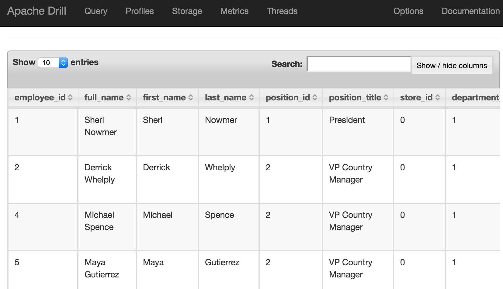
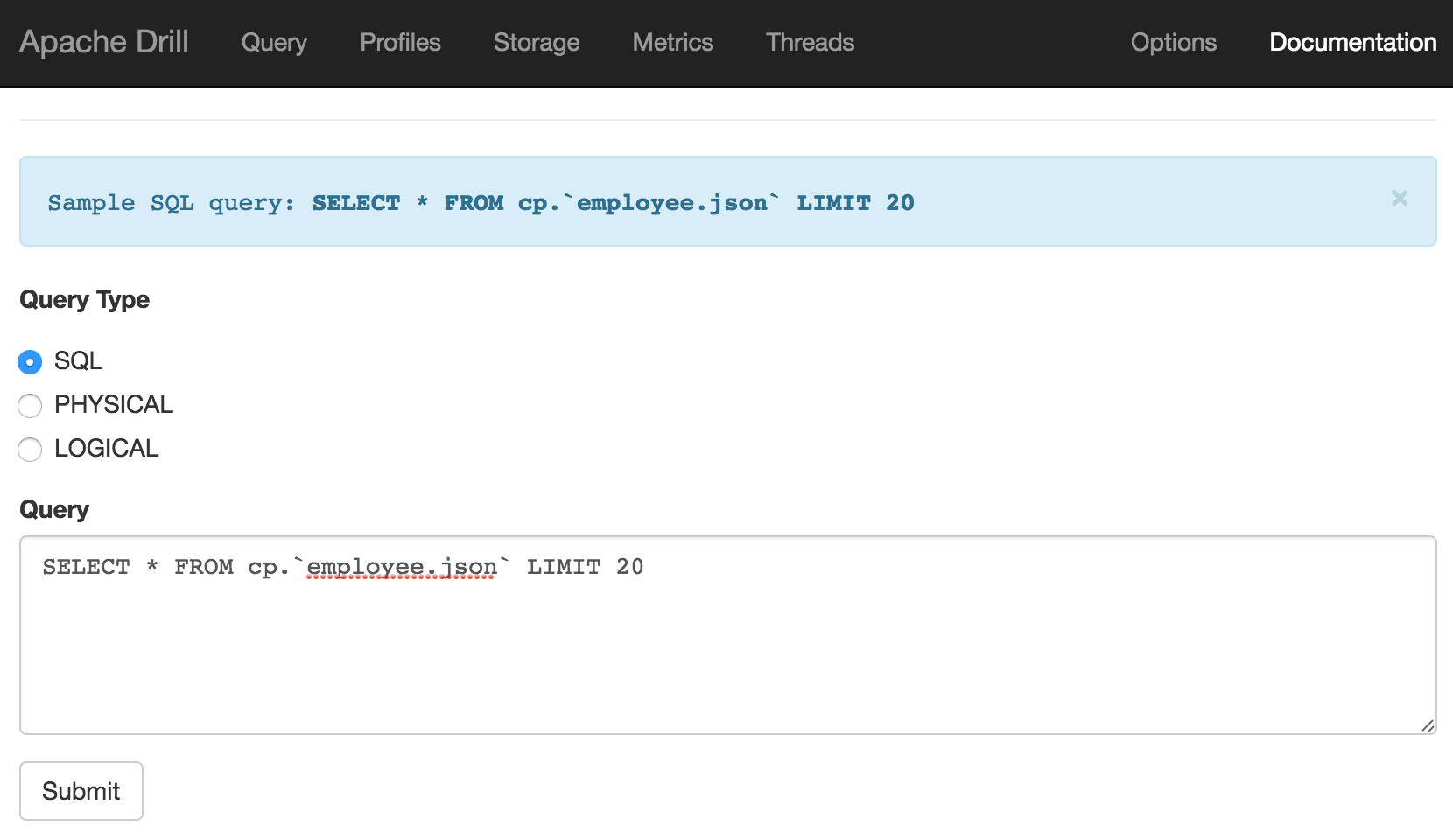
There's a built in dataset that you can use for testing:

USE cp;
SELECT employee_id, first_name FROM `employee.json` limit 5;

This should return five rows, in a very familiar environment if you're used to using SQL*Plus and similar tools:

0: jdbc:drill:zk=local> USE cp;
+-------+---------------------------------+
|  ok   |             summary             |
+-------+---------------------------------+
| true  | Default schema changed to [cp]  |
+-------+---------------------------------+
1 row selected (1.776 seconds)
0: jdbc:drill:zk=local>     SELECT employee_id, first_name FROM `employee.json` limit 5;
+--------------+-------------+
| employee_id  | first_name  |
+--------------+-------------+
| 1            | Sheri       |
| 2            | Derrick     |
| 4            | Michael     |
| 5            | Maya        |
| 6            | Roberta     |
+--------------+-------------+
5 rows selected (3.624 seconds)

So far, so SQL, so relational - so familiar, really. Where Apache Drill starts to deviate from the obvious is its use of storage handlers. In the above query cp is the 'database' that we're running our query against, but this is in fact a "classpath" (hence "cp") storage handler that's defined by default. Within a 'database' there are 'schemas' which are sub-configurations of the storage handler. We'll have a look at viewing and defining these later on. For now, it's useful to know that you can also list out the available databases:

0: jdbc:drill:zk=local> show databases;
+---------------------+
|     SCHEMA_NAME     |
+---------------------+
| INFORMATION_SCHEMA  |
| cp.default          |
| dfs.default         |
| dfs.root            |
| dfs.tmp             |
| sys                 |
+---------------------+

Note databases command is a synonym for schemas; it's the <database>.<schema> that's returned for both. In Apache Drill the backtick is used to enclose identifiers (such as schema names, column names, and so on), and it's quite particular about it. For example, this is valid:

0: jdbc:drill:zk=local> USE `cp.default`;
+-------+-----------------------------------------+
|  ok   |                 summary                 |
+-------+-----------------------------------------+
| true  | Default schema changed to [cp.default]  |
+-------+-----------------------------------------+
1 row selected (0.171 seconds)

whilst this isn't:

0: jdbc:drill:zk=local> USE cp.default;
Error: PARSE ERROR: Encountered ". default" at line 1, column 7.
Was expecting one of:
<EOF>
"." <IDENTIFIER> ...
"." <QUOTED_IDENTIFIER> ...
"." <BACK_QUOTED_IDENTIFIER> ...
"." <BRACKET_QUOTED_IDENTIFIER> ...
"." <UNICODE_QUOTED_IDENTIFIER> ...
"." "*" ...

SQL Query USE cp.default

This is because default is a reserved word, and hence must be quoted. Hence, you can also use

0: jdbc:drill:zk=local> use cp.`default`;

but not

0: jdbc:drill:zk=local> use `cp`.default;

Querying JSON data

On the Apache Drill website there's some useful tutorials, including one using data provided by Yelp . This was the dataset that originally got me looking at Drill, since I was using it as an input to Big Data Discovery (BDD) but struggling on two counts. First up was how best to define a suitable Hive table over it in order to ingest it to BDD. Following from this was trying to understand what value there might be in the data which would drive how long to spend perfecting the way in which I exposed the data in Hive. The examples below show the kind of complications that complex JSON can introduce when queried in a tabular fashion.

First up, querying a JSON file, with the schema inferred automagically. Pretty cool.

0: jdbc:drill:zk=local> select * from `/user/oracle/incoming/yelp/tip_json/yelp_academic_dataset_tip.json` limit 5;
+---------+------+-------------+-------+------+------+
| user_id | text | business_id | likes | date | type |
+---------+------+-------------+-------+------+------+
| -6rEfobYjMxpUWLNxszaxQ | Don't waste your time. | cE27W9VPgO88Qxe4ol6y_g | 0 | 2013-04-18 | tip |
| EZ0r9dKKtEGVx2CdnowPCw | Your GPS will not allow you to find this place. Put Rankin police department in instead. They are directly across the street. | mVHrayjG3uZ_RLHkLj-AMg | 1 | 2013-01-06 | tip |
| xb6zEQCw9I-Gl0g06e1KsQ | Great drink specials! | KayYbHCt-RkbGcPdGOThNg | 0 | 2013-12-03 | tip |
| QawZN4PSW7ng_9SP7pjsVQ | Friendly staff, good food, great beer selection, and relaxing atmosphere | KayYbHCt-RkbGcPdGOThNg | 0 | 2015-07-08 | tip |
| MLQre1nvUtW-RqMTc4iC9A | Beautiful restoration. | 1_lU0-eSWJCRvNGk78Zh9Q | 0 | 2015-10-25 | tip |
+---------+------+-------------+-------+------+------+
5 rows selected (2.341 seconds)

We can use standard SQL aggregations such as COUNT:

0: jdbc:drill:zk=local> select count(*) from `/user/oracle/incoming/yelp/tip_json/yelp_academic_dataset_tip.json`;
+---------+
| EXPR$0  |
+---------+
| 591864  |
+---------+
1 row selected (4.495 seconds)

as well as GROUP BY operation:

0: jdbc:drill:zk=local> select `date`,count(*) as tip_count from `/user/oracle/incoming/yelp/tip_json/yelp_academic_dataset_tip.json` group by `date` order by 2 desc limit 5;
+-------------+------------+
|    date     | tip_count  |
+-------------+------------+
| 2012-07-21  | 719        |
| 2012-05-19  | 718        |
| 2012-08-04  | 699        |
| 2012-06-23  | 690        |
| 2012-07-28  | 682        |
+-------------+------------+
5 rows selected (7.111 seconds)

Digging into the data a bit, we can see that it's not entirely flat - note, for example, the hours column, which is a nested JSON object:

0: jdbc:drill:zk=local> select full_address,city,hours from `/user/oracle/incoming/yelp/business_json` b limit 5;
+--------------+------+-------+
| full_address | city | hours |
+--------------+------+-------+
| 4734 Lebanon Church Rd
Dravosburg, PA 15034 | Dravosburg | {"Friday":{"close":"21:00","open":"11:00"},"Tuesday":{"close":"21:00","open":"11:00"},"Thursday":{"close":"21:00","open":"11:00"},"Wednesday":{"close":"21:00","open":"11:00"},"Monday":{"close":"21:00","open":"11:00"},"Sunday":{},"Saturday":{}} |
| 202 McClure St
Dravosburg, PA 15034 | Dravosburg | {"Friday":{},"Tuesday":{},"Thursday":{},"Wednesday":{},"Monday":{},"Sunday":{},"Saturday":{}} |
| 1 Ravine St
Dravosburg, PA 15034 | Dravosburg | {"Friday":{},"Tuesday":{},"Thursday":{},"Wednesday":{},"Monday":{},"Sunday":{},"Saturday":{}} |
| 1530 Hamilton Rd
Bethel Park, PA 15234 | Bethel Park | {"Friday":{},"Tuesday":{},"Thursday":{},"Wednesday":{},"Monday":{},"Sunday":{},"Saturday":{}} |
| 301 South Hills Village
Pittsburgh, PA 15241 | Pittsburgh | {"Friday":{"close":"17:00","open":"10:00"},"Tuesday":{"close":"21:00","open":"10:00"},"Thursday":{"close":"17:00","open":"10:00"},"Wednesday":{"close":"21:00","open":"10:00"},"Monday":{"close":"21:00","open":"10:00"},"Sunday":{"close":"18:00","open":"11:00"},"Saturday":{"close":"21:00","open":"10:00"}} |
+--------------+------+-------+
5 rows selected (0.721 seconds)
0: jdbc:drill:zk=local>

With Apache Drill we can simply use dot notation to access nested values. It's necessary to alias the table (b in this example) when you're doing this:

0: jdbc:drill:zk=local> select b.hours from `/user/oracle/incoming/yelp/business_json` b limit 1;
+-------+
| hours |
+-------+
| {"Friday":{"close":"21:00","open":"11:00"},"Tuesday":{"close":"21:00","open":"11:00"},"Thursday":{"close":"21:00","open":"11:00"},"Wednesday":{"close":"21:00","open":"11:00"},"Monday":{"close":"21:00","open":"11:00"},"Sunday":{},"Saturday":{}} |
+-------+

Nested objects can themselves be nested - not a problem with Apache Drill, we just chain the dot notation further:

0: jdbc:drill:zk=local> select b.hours.Friday from `/user/oracle/incoming/yelp/business_json` b limit 1;
+-----------------------------------+
|              EXPR$0               |
+-----------------------------------+
| {"close":"21:00","open":"11:00"}  |
+-----------------------------------+
1 row selected (0.238 seconds)

Note the use of backtick (`) to quote the reserved open and close keywords:

0: jdbc:drill:zk=local> select b.hours.Friday.`open`,b.hours.Friday.`close` from `/user/oracle/incoming/yelp/business_json` b limit 1;
+---------+---------+
| EXPR$0  | EXPR$1  |
+---------+---------+
| 11:00   | 21:00   |
+---------+---------+
1 row selected (0.58 seconds)

Nested columns are proper objects in their own right in the query, and can be used as predicates too:

0: jdbc:drill:zk=local> select b.name,b.full_address,b.hours.Friday.`open` from `/user/oracle/incoming/yelp/business_json` b where b.hours.Friday.`open` = '11:00' limit 5;
+------------------------+------------------------------------------------+---------+
|          name          |                  full_address                  | EXPR$2  |
+------------------------+------------------------------------------------+---------+
| Mr Hoagie              | 4734 Lebanon Church Rd
Dravosburg, PA 15034    | 11:00   |
| Alexion's Bar & Grill  | 141 Hawthorne St
Greentree
Carnegie, PA 15106  | 11:00   |
| Rocky's Lounge         | 1201 Washington Ave
Carnegie, PA 15106         | 11:00   |
| Papa J's               | 200 E Main St
Carnegie
Carnegie, PA 15106      | 11:00   |
| Italian Village Pizza  | 2615 Main St
Homestead, PA 15120               | 11:00   |
+------------------------+------------------------------------------------+---------+
5 rows selected (0.404 seconds)

You'll notice in the above output that the full_address field has line breaks in -- we can just use a SQL Function to replace line breaks with commas:

0: jdbc:drill:zk=local> select b.name,regexp_replace(b.full_address,'\n',','),b.hours.Friday.`open` from `/user/oracle/incoming/yelp/business_json` b where b.hours.Friday.`open` = '11:00' limit 5;
+------------------------+------------------------------------------------+---------+
|          name          |                     EXPR$1                     | EXPR$2  |
+------------------------+------------------------------------------------+---------+
| Mr Hoagie              | 4734 Lebanon Church Rd,Dravosburg, PA 15034    | 11:00   |
| Alexion's Bar & Grill  | 141 Hawthorne St,Greentree,Carnegie, PA 15106  | 11:00   |
| Rocky's Lounge         | 1201 Washington Ave,Carnegie, PA 15106         | 11:00   |
| Papa J's               | 200 E Main St,Carnegie,Carnegie, PA 15106      | 11:00   |
| Italian Village Pizza  | 2615 Main St,Homestead, PA 15120               | 11:00   |
+------------------------+------------------------------------------------+---------+
5 rows selected (1.346 seconds)

Query Federation

So Apache Drill enables you to run SQL queries against data in a multitude of formats and locations, which is rather useful in itself. But even better than that, it lets you federate these sources in a single query. Here's an example of joining between data in HDFS and Oracle:

0: jdbc:drill:zk=local> select X.text,
. . . . . . . . . . . > Y.NAME
. . . . . . . . . . . > from hdfs.`/user/oracle/incoming/yelp/tip_json/yelp_academic_dataset_tip.json` X
. . . . . . . . . . . > inner join ora.MOVIEDEMO.YELP_BUSINESS Y
. . . . . . . . . . . > on X.business_id = Y.BUSINESS_ID
. . . . . . . . . . . > where Y.NAME = 'Chick-fil-A'
. . . . . . . . . . . > limit 5;
+--------------------------------------------------------------------+--------------+
|                                text                                |     NAME     |
+--------------------------------------------------------------------+--------------+
| It's daddy daughter date night here and they go ALL OUT!           | Chick-fil-A  |
| Chicken minis!  The best part of waking up Saturday mornings.  :)  | Chick-fil-A  |
| Nice folks as always unlike those ghetto joints                    | Chick-fil-A  |
| Great clean and delicious chicken sandwiches!                      | Chick-fil-A  |
| Spicy Chicken with lettuce, tomato, and pepperjack cheese FTW!     | Chick-fil-A  |
+--------------------------------------------------------------------+--------------+
5 rows selected (3.234 seconds)

You can define a view over this:

0: jdbc:drill:zk=local> create or replace view dfs.tmp.yelp_tips as select X.text as tip_text, Y.NAME as business_name from hdfs.`/user/oracle/incoming/yelp/tip_json/yelp_academic_dataset_tip.json` X inner join ora.MOVIEDEMO.YELP_BUSINESS Y on X.business_id = Y.BUSINESS_ID ;
+-------+-------------------------------------------------------------+
|  ok   |                           summary                           |
+-------+-------------------------------------------------------------+
| true  | View 'yelp_tips' replaced successfully in 'dfs.tmp' schema  |
+-------+-------------------------------------------------------------+
1 row selected (0.574 seconds)
0: jdbc:drill:zk=local> describe dfs.tmp.yelp_tips;
+----------------+--------------------+--------------+
|  COLUMN_NAME   |     DATA_TYPE      | IS_NULLABLE  |
+----------------+--------------------+--------------+
| tip_text       | ANY                | YES          |
| business_name  | CHARACTER VARYING  | YES          |
+----------------+--------------------+--------------+
2 rows selected (0.756 seconds)

and then query it as any regular object:

0: jdbc:drill:zk=local> select tip_text,business_name from dfs.tmp.yelp_tips where business_name like '%Grill' limit 5;
+------+------+
| text | NAME |
+------+------+
| Great drink specials! | Alexion's Bar & Grill |
| Friendly staff, good food, great beer selection, and relaxing atmosphere | Alexion's Bar & Grill |
| Pretty quiet here... | Uno Pizzeria & Grill |
| I recommend this location for quick lunches. 10 min or less lunch menu. Soup bar ( all you can eat)  the broccoli cheddar soup is delicious. | Uno Pizzeria & Grill |
| Instead of pizza, come here for dessert. The deep dish sundae is really good. | Uno Pizzeria & Grill |
+------+------+
5 rows selected (3.272 seconds)

Querying Twitter JSON data

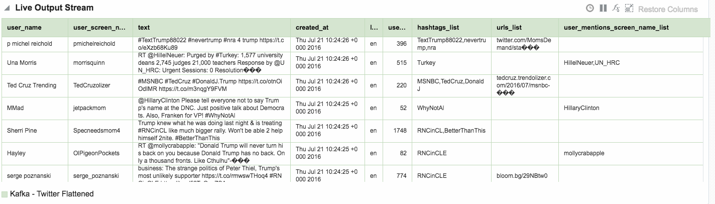
Here's an example of using Drill to query a local file holding some Twitter data. You can download the file here if you want to try querying it yourself.

To start with I switched to using the dfs storage plugin:

0: jdbc:drill:zk=local> use dfs;
+-------+----------------------------------+
|  ok   |             summary              |
+-------+----------------------------------+
| true  | Default schema changed to [dfs]  |
+-------+----------------------------------+

And then tried a select against the file. Note the limit 5 clause - very useful when you're just examining the structure of a file.

0: jdbc:drill:zk=local> select * from `/user/oracle/incoming/twitter/geo_tweets.json` limit 5;
Error: DATA_READ ERROR: Error parsing JSON - Unexpected end-of-input within/between OBJECT entries

File  /user/oracle/incoming/twitter/geo_tweets.json
Record  2819
Column  3503
Fragment 0:0

An error? That's not supposed to happen. I've got a JSON file, right? It turns out the JSON file is one complete JSON object per line. Except that it's not on the last record. Note the record count given in the error above - 2819:

[oracle@bigdatalite ~]$ wc -l geo_tweets.json
2818 geo_tweets.json

So the file only has 2818 complete lines. Hmmm. Let's take a look at that record, using a head/tail bash combo :

[oracle@bigdatalite ~]$ head -n 2819 geo_tweets.json |tail -n1
{"created_at":"Sun Jul 24 21:00:44 +0000 2016","id":757319630432067584,"id_str":"757319630432067584","text":"And now @HillaryClinton hires @DWStweets: Honorary Campaign Manager across the USA #corruption #hillarysamerica  https://t.co/8jAGUu6w2f","source":"<a href=\"http://www.handmark.com\" rel=\"nofollow\">TweetCaster for iOS</a>","truncated":false,"in_reply_to_status_id":null,"in_reply_to_status_id_str":null,"in_reply_to_user_id":null,"in_reply_to_user_id_str":null,"in_reply_to_screen_name":null,"user":{"id":2170786369,"id_str":"2170786369","name":"Patricia Weber","screen_name":"InnieBabyBoomer","location":"Williamsburg, VA","url":"http://lovesrantsandraves.blogspot.com/","description":"Baby Boomer, Swing Voter, Conservative, Spiritual, #Introvert, Wife, Grandma, Italian, ♥ Books, Cars, Ferrari, F1 Race♥  #tcot","protected":false,"verified":false,"followers_count":861,"friends_count":918,"listed_count":22,"favourites_count":17,"statuses_count":2363,"created_at":"Sat Nov 02 19:13:06 +0000 2013","utc_offset":null,"time_zone":null,"geo_enabled":true,"lang":"en","contributors_enabled":false,"is_translator":false,"profile_background_color":"C0DEED","profile_background_image_url":"http://pbs.twimg.com/profile_background_images/378800000107659131/3589f

That's the complete data in the file - so Drill is right - the JSON is corrupted. If we drop that last record and create a new file (geo_tweets.fixed.json)

head -n2818 geo_tweets.json > geo_tweets.fixed.json

and query it again, we get something!

0: jdbc:drill:zk=local>  select text from `/users/rmoff/data/geo_tweets.fixed.json` limit 5;
+------+
| text |
+------+
| Vancouver trends now: Trump, Evander Kane, Munich, 2016HCC and dcc16. https://t.co/joI9GMfRim |
| We're #hiring! Click to apply: Bench Jeweler - SEC Oracle & Wetmore - https://t.co/Oe2SHaL0Hh #Job #SkilledTrade #Tucson, AZ #Jobs |
| Donald Trump accepted the Republican nomination last night. Isis claimed responsibility. |
| Obama: "We must stand together and stop terrorism"
Trump: "We don't want these people in our country"
� |
| Someone built a wall around Trump's star on the Hollywood Walk of Fame. #lol #nowthatsfunny @… https://t.co/qHWuJXnzbw |
+------+
5 rows selected (0.246 seconds)

text here being one of the json fields. I could do a select * but it's not so intelligable:

0: jdbc:drill:zk=local>  select * from `/users/rmoff/data/geo_tweets.fixed.json` limit 5;
+------------+----+--------+------+--------+-----------+------+-----+-------------+-------+-----------------+---------------+----------------+----------+-----------+-----------+--------------------+--------------+------+--------------+----------+------------+-----------+------------------+----------------------+--------------------+-------------------+-----------------------+---------------------+-----------------+------------+---------------+---------------+------------+-----------+--------------------------------+-----------+----------+----------------+-------------------+---------------------------------+-----------------------+---------------------------+---------------------+-------------------------+-------------------------+------------------+-----------------------+------------------+----------------------+---------------+
| created_at | id | id_str | text | source | truncated | user | geo | coordinates | place | is_quote_status | retweet_count | favorite_count | entities | favorited | retweeted | possibly_sensitive | filter_level | lang | timestamp_ms | @version | @timestamp | user_name | user_screen_name | user_followers_count | user_friends_count | user_listed_count | user_favourites_count | user_statuses_count | user_created_at | place_name | place_country | hashtags_list | urls_array | urls_list | user_mentions_screen_name_list | longitude | latitude | hashtags_array | extended_entities | user_mentions_screen_name_array | in_reply_to_status_id | in_reply_to_status_id_str | in_reply_to_user_id | in_reply_to_user_id_str | in_reply_to_screen_name | retweeted_status | retweeted_screen_name | quoted_status_id | quoted_status_id_str | quoted_status |
+------------+----+--------+------+--------+-----------+------+-----+-------------+-------+-----------------+---------------+----------------+----------+-----------+-----------+--------------------+--------------+------+--------------+----------+------------+-----------+------------------+----------------------+--------------------+-------------------+-----------------------+---------------------+-----------------+------------+---------------+---------------+------------+-----------+--------------------------------+-----------+----------+----------------+-------------------+---------------------------------+-----------------------+---------------------------+---------------------+-------------------------+-------------------------+------------------+-----------------------+------------------+----------------------+---------------+
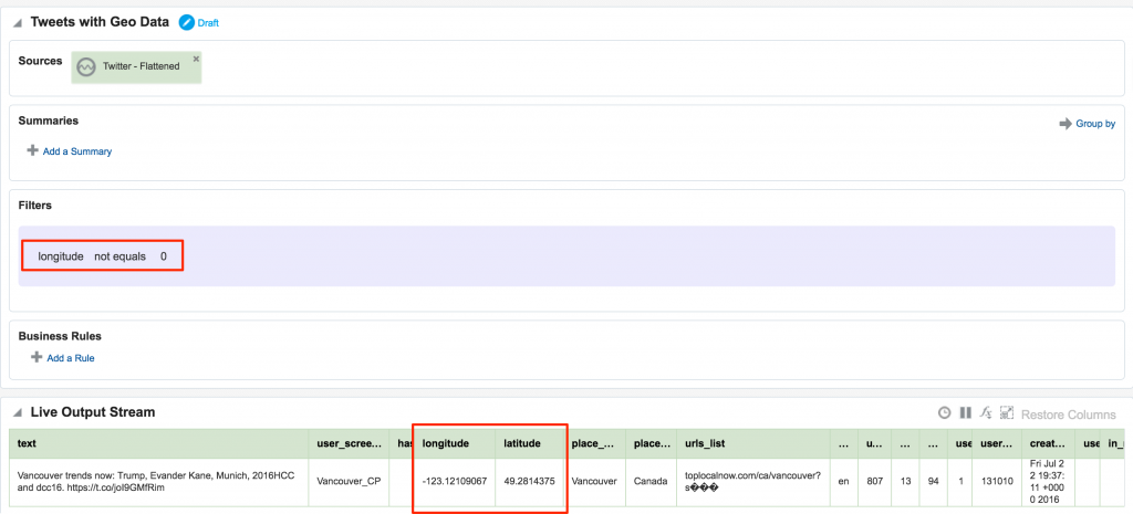
| Fri Jul 22 19:37:11 +0000 2016 | 756573827589545984 | 756573827589545984 | Vancouver trends now: Trump, Evander Kane, Munich, 2016HCC and dcc16. https://t.co/joI9GMfRim | <a href="http://dlvr.it" rel="nofollow">dlvr.it</a> | false | {"id":67898674,"id_str":"67898674","name":"Vancouver Press","screen_name":"Vancouver_CP","location":"Vancouver, BC","url":"http://vancouver.cityandpress.com/","description":"Latest news from Vancouver. Updates are frequent.","protected":false,"verified":false,"followers_count":807,"friends_count":13,"listed_count":94,"favourites_count":1,"statuses_count":131010,"created_at":"Sat Aug 22 14:25:37 +0000 2009","utc_offset":-25200,"time_zone":"Pacific Time (US & Canada)","geo_enabled":true,"lang":"en","contributors_enabled":false,"is_translator":false,"profile_background_color":"FFFFFF","profile_background_image_url":"http://abs.twimg.com/images/themes/theme1/bg.png","profile_background_image_url_https":"https://abs.twimg.com/images/themes/theme1/bg.png","profile_background_tile":false,"profile_link_color":"8A1C3B","profile_sidebar_border_color":"FFFFFF","profile_sidebar_fill_color":"FFFFFF","profile_text_color":"2A2C31","profile_use_background_image":false,"profile_image_url":"http://pbs.twimg.com/profile_images/515841109553983490/_t0QWPco_normal.png","profile_image_url_https":"https://pbs.twimg.com/profile_images/515841109553983490/_t0QWPco_normal.png","profile_banner_url":"https://pbs.twimg.com/profile_banners/67898674/1411821103","default_profile":false,"default_profile_image":false} | {"type":"Point","coordinates":[49.2814375,-123.12109067]} | {"type":"Point","coordinates":[-123.12109067,49.2814375]} | {"id":"1e5cb4d0509db554","url":"https://api.twitter.com/1.1/geo/id/1e5cb4d0509db554.json","place_type":"city","name":"Vancouver","full_name":"Vancouver, British Columbia","country_code":"CA","country":"Canada","bounding_box":{"type":"Polygon","coordinates":[[[-123.224215,49.19854],[-123.224215,49.316738],[-123.022947,49.316738],[-123.022947,49.19854]]]},"attributes":{}} | false | 0 | 0 | {"urls":[{"url":"https://t.co/joI9GMfRim","expanded_url":"http://toplocalnow.com/ca/vancouver?section=trends","display_url":"toplocalnow.com/ca/vancouver?s…","indices":[70,93]}],"hashtags":[],"user_mentions":[],"media":[],"symbols":[]} | false | false | false | low | en | 1469216231616 | 1 | 2016-07-22T19:37:11.000Z | Vancouver Press | Vancouver_CP | 807 | 13 | 94 | 1 | 131010 | Sat Aug 22 14:25:37 +0000 2009 | Vancouver | Canada |  | ["toplocalnow.com/ca/vancouver?s…"] | toplocalnow.com/ca/vancouver?s… |  | -123.12109067 | 49.2814375 | [] | {"media":[]} | [] | null | null | null | null | null | {"user":{},"entities":{"user_mentions":[],"media":[],"hashtags":[],"urls":[]},"extended_entities":{"media":[]},"quoted_status":{"user":{},"entities":{"hashtags":[],"user_mentions":[],"media":[],"urls":[]},"extended_entities":{"media":[]}}} | null | null | null | {"user":{},"entities":{"user_mentions":[],"media":[],"urls":[],"hashtags":[]},"extended_entities":{"media":[]},"place":{"bounding_box":{"coordinates":[]},"attributes":{}},"geo":{"coordinates":[]},"coordinates":{"coordinates":[]}} |

Within the twitter data there's root-level fields, such as text, as well as nested ones such as information about the tweeter in the user field. As we saw above you reference nested fields using dot notation. Now's a good time to point out a couple of common mistakes that you may encounter. The first is not quoting reserved words, and is the first thing to check for if you get an error such as Encountered ".":

0: jdbc:drill:zk=local>  select user.screen_name,text from `/users/rmoff/data/geo_tweets.fixed.json` limit 5;
Error: PARSE ERROR: Encountered "." at line 1, column 12.
[...]

Second is declaring the table alias when using dot notation - if you don't then Apache Drill thinks that the parent column is actually the table name (VALIDATION ERROR: [...] Table 'user' not found):

0: jdbc:drill:zk=local>  select `user`.screen_name,text from dfs.`/users/rmoff/data/geo_tweets.fixed.json` limit 5;
Aug 10, 2016 11:16:45 PM org.apache.calcite.sql.validate.SqlValidatorException <init>
SEVERE: org.apache.calcite.sql.validate.SqlValidatorException: Table 'user' not found
Aug 10, 2016 11:16:45 PM org.apache.calcite.runtime.CalciteException <init>
SEVERE: org.apache.calcite.runtime.CalciteContextException: From line 1, column 8 to line 1, column 13: Table 'user' not found
Error: VALIDATION ERROR: From line 1, column 8 to line 1, column 13: Table 'user' not found

SQL Query null

[Error Id: 1427fd23-e180-40be-a751-b6f1f838233a on 192.168.56.1:31010] (state=,code=0)

With those mistakes fixed, we can see the user's screenname:

0: jdbc:drill:zk=local>  select tweets.`user`.`screen_name` as user_screen_name,text from dfs.`/users/rmoff/data/geo_tweets.fixed.json` tweets limit 2;
+------------------+------+
| user_screen_name | text |
+------------------+------+
| Vancouver_CP     | Vancouver trends now: Trump, Evander Kane, Munich, 2016HCC and dcc16. https://t.co/joI9GMfRim |
| tmj_TUC_skltrd   | We're #hiring! Click to apply: Bench Jeweler - SEC Oracle & Wetmore - https://t.co/Oe2SHaL0Hh #Job #SkilledTrade #Tucson, AZ #Jobs |
+------------------+------+
2 rows selected (0.256 seconds)
0: jdbc:drill:zk=local>

As well as nested objects, JSON supports arrays. An example of this in twitter data is hashtags, or URLs, both of which there can be zero, one, or many of in a given tweet.

0: jdbc:drill:zk=local>  select tweets.entities.hashtags from dfs.`/users/rmoff/data/geo_tweets.fixed.json` tweets limit 5;
+--------+
| EXPR$0 |
+--------+
| [] |
| [{"text":"hiring","indices":[6,13]},{"text":"Job","indices":[98,102]},{"text":"SkilledTrade","indices":[103,116]},{"text":"Tucson","indices":[117,124]},{"text":"Jobs","indices":[129,134]}] |
| [] |
| [] |
| [{"text":"lol","indices":[72,76]},{"text":"nowthatsfunny","indices":[77,91]}] |
+--------+
5 rows selected (0.286 seconds)

Using the FLATTEN function each array entry becomes a new row, thus:

0: jdbc:drill:zk=local>  select flatten(tweets.entities.hashtags) from dfs.`/users/rmoff/data/geo_tweets.fixed.json` tweets limit 5;
+----------------------------------------------+
|                    EXPR$0                    |
+----------------------------------------------+
| {"text":"hiring","indices":[6,13]}           |
| {"text":"Job","indices":[98,102]}            |
| {"text":"SkilledTrade","indices":[103,116]}  |
| {"text":"Tucson","indices":[117,124]}        |
| {"text":"Jobs","indices":[129,134]}          |
+----------------------------------------------+
5 rows selected (0.139 seconds)

Note that the limit 5 clause is showing only the first five array instances, which is actually just hashtags from the first tweet in the above list.

To access the text of the hashtag we use a subquery and the dot notation to access the text field:

0: jdbc:drill:zk=local> select ent_hashtags.hashtags.text from (select flatten(tweets.entities.hashtags) as hashtags from dfs.`/users/rmoff/data/geo_tweets.fixed.json` tweets) as ent_hashtags limit 5;
+---------------+
|    EXPR$0     |
+---------------+
| hiring        |
| Job           |
| SkilledTrade  |
| Tucson        |
| Jobs          |
+---------------+
5 rows selected (0.168 seconds)

This can be made more readable by using Common Table Expressions (CTE, also known as subquery factoring) for the same result:

0: jdbc:drill:zk=local> with ent_hashtags as (select flatten(tweets.entities.hashtags) as hashtags from dfs.`/users/rmoff/data/geo_tweets.fixed.json` tweets)
. . . . . . . . . . . > select ent_hashtags.hashtags.text from ent_hashtags
. . . . . . . . . . . > limit 5;
+---------------+
|    EXPR$0     |
+---------------+
| hiring        |
| Job           |
| SkilledTrade  |
| Tucson        |
| Jobs          |
+---------------+
5 rows selected (0.253 seconds)

Combining the flattened array with existing fields enables us to see things like a list of tweets with their associated hashtags:

0: jdbc:drill:zk=local> with tmp as ( select flatten(tweets.entities.hashtags) as hashtags,tweets.text,tweets.`user`.screen_name as user_screen_name from dfs.`/users/rmoff/data/geo_tweets.fixed.json` tweets) select tmp.user_screen_name,tmp.text,tmp.hashtags.text as hashtag from tmp limit 10;
+------------------+------+---------+
| user_screen_name | text | hashtag |
+------------------+------+---------+
| tmj_TUC_skltrd | We're #hiring! Click to apply: Bench Jeweler - SEC Oracle & Wetmore - https://t.co/Oe2SHaL0Hh #Job #SkilledTrade #Tucson, AZ #Jobs | hiring |
| tmj_TUC_skltrd | We're #hiring! Click to apply: Bench Jeweler - SEC Oracle & Wetmore - https://t.co/Oe2SHaL0Hh #Job #SkilledTrade #Tucson, AZ #Jobs | Job |
| tmj_TUC_skltrd | We're #hiring! Click to apply: Bench Jeweler - SEC Oracle & Wetmore - https://t.co/Oe2SHaL0Hh #Job #SkilledTrade #Tucson, AZ #Jobs | SkilledTrade |
| tmj_TUC_skltrd | We're #hiring! Click to apply: Bench Jeweler - SEC Oracle & Wetmore - https://t.co/Oe2SHaL0Hh #Job #SkilledTrade #Tucson, AZ #Jobs | Tucson |
| tmj_TUC_skltrd | We're #hiring! Click to apply: Bench Jeweler - SEC Oracle & Wetmore - https://t.co/Oe2SHaL0Hh #Job #SkilledTrade #Tucson, AZ #Jobs | Jobs |
| johnmayberry | Someone built a wall around Trump's star on the Hollywood Walk of Fame. #lol #nowthatsfunny @… https://t.co/qHWuJXnzbw | lol |
| johnmayberry | Someone built a wall around Trump's star on the Hollywood Walk of Fame. #lol #nowthatsfunny @… https://t.co/qHWuJXnzbw | nowthatsfunny |
| greensboro_nc | #WinstonSalem Time and place announced for Donald Trump's visit to… https://t.co/6OVl7crshw #ws @winston_salem_ https://t.co/l5h220otj4 | WinstonSalem |
| greensboro_nc | #WinstonSalem Time and place announced for Donald Trump's visit to… https://t.co/6OVl7crshw #ws @winston_salem_ https://t.co/l5h220otj4 | ws |
| trendinaliaSG | 6. Hit The Stage
7. TTTT
8. Demi Lovato
9. Beijing
10. Donald Trump

2016/7/23 03:36 SGT #trndnl https://t.co/psP0GzBgZB | trndnl |
+------------------+------+---------+
10 rows selected (0.166 seconds)

We can also filter based on hashtag:

0: jdbc:drill:zk=local> with tmp as ( select flatten(tweets.entities.hashtags) as hashtags,tweets.text,tweets.`user`.screen_name as user_screen_name from dfs.`/users/rmoff/data/geo_tweets.fixed.json` tweets) select tmp.user_screen_name,tmp.text,tmp.hashtags.text as hashtag from tmp where tmp.hashtags.text = 'Job' limit 5;
+------------------+------+---------+
| user_screen_name | text | hashtag |
+------------------+------+---------+
| tmj_TUC_skltrd | We're #hiring! Click to apply: Bench Jeweler - SEC Oracle & Wetmore - https://t.co/Oe2SHaL0Hh #Job #SkilledTrade #Tucson, AZ #Jobs | Job |
| tmj_VAL_health | Want to work at Genesis Rehab Services? We're #hiring in #Clinton, MD! Click for details: https://t.co/4lt7I4gMZk #Job #Healthcare #Jobs | Job |
| tmj_in_retail | Want to work in #Clinton, IN? View our latest opening: https://t.co/UiimnlubYs #Job #Retail #Jobs #Hiring #CareerArc | Job |
| tmj_la_hrta | Want to work at SONIC Drive-In? We're #hiring in #Clinton, LA! Click for details: https://t.co/aQ1FrWc7iR #Job #SONIC #Hospitality #Jobs | Job |
| tmj_ia_hrta | We're #hiring! Click to apply: Department Manager - https://t.co/SnoKcwwHFk #Job #Hospitality #Clinton, IA #Jobs #CareerArc | Job |
+------------------+------+---------+
5 rows selected (0.207 seconds)

as well as summarise hashtag counts:

0: jdbc:drill:zk=local> with ent_hashtags as (select flatten(tweets.entities.hashtags) as hashtags from dfs.`/users/rmoff/data/geo_tweets.fixed.json` tweets)
. . . . . . . . . . . > select ent_hashtags.hashtags.text,count(ent_hashtags.hashtags.text) from ent_hashtags
. . . . . . . . . . . > group by ent_hashtags.hashtags.text
. . . . . . . . . . . > order by 2 desc;
+-----------------------------+---------+
|           EXPR$0            | EXPR$1  |
+-----------------------------+---------+
| Trump                       | 365     |
| trndnl                      | 176     |
| job                         | 170     |
| Hiring                      | 127     |
| Clinton                     | 108     |
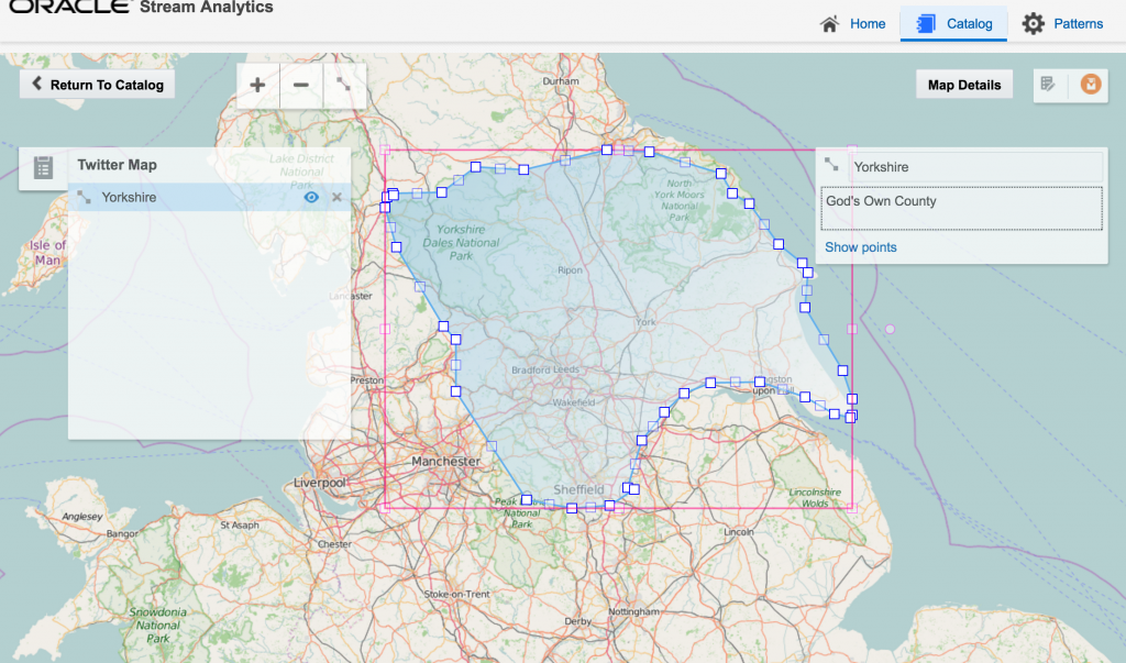
| Yorkshire                   | 100     |
| CareerArc                   | 100     |
[...]

To filter out records that may not have array values (such as hashtags, which not every tweet has) and without with the query may fail, use IS NOT NULL against an attribute of first index of the array:

0: jdbc:drill:zk=local> select tweets.entities.hashtags from dfs.`/users/rmoff/data/geo_tweets.fixed.json` tweets where tweets.entities.hashtags[0].text is not null limit 5;
+--------+
| EXPR$0 |
+--------+
| [{"text":"hiring","indices":[6,13]},{"text":"Job","indices":[98,102]},{"text":"SkilledTrade","indices":[103,116]},{"text":"Tucson","indices":[117,124]},{"text":"Jobs","indices":[129,134]}] |
| [{"text":"lol","indices":[72,76]},{"text":"nowthatsfunny","indices":[77,91]}] |
| [{"text":"WinstonSalem","indices":[0,13]},{"text":"ws","indices":[92,95]}] |
| [{"text":"trndnl","indices":[89,96]}] |
| [{"text":"trndnl","indices":[92,99]}] |
+--------+
5 rows selected (0.187 seconds)

If you try and compare the array itself, it doesn't work:

0: jdbc:drill:zk=local> select tweets.entities.hashtags from dfs.`/users/rmoff/data/geo_tweets.fixed.json` tweets where tweets.entities.hashtags is not null limit 5;
Error: SYSTEM ERROR: SchemaChangeException: Failure while trying to materialize incoming schema.  Errors:

Error in expression at index -1.  Error: Missing function implementation: [isnotnull(MAP-REPEATED)].  Full expression: --UNKNOWN EXPRESSION--..

Fragment 0:0

[Error Id: 99ac12aa-f6b4-4692-b815-8f483da682c4 on 192.168.56.1:31010] (state=,code=0)

The above example demonstrates using array indexing, which is an alternative to FLATTEN for accessing individual objects in the array if you know they're going to exist:

0: jdbc:drill:zk=local> select tweets.entities.hashtags[0].text as first_hashtag,text from dfs.`/users/rmoff/data/geo_tweets.fixed.json` tweets where tweets.entities.hashtags[0].text is not null limit 5;
+---------------+------+
| first_hashtag | text |
+---------------+------+
| hiring | We're #hiring! Click to apply: Bench Jeweler - SEC Oracle & Wetmore - https://t.co/Oe2SHaL0Hh #Job #SkilledTrade #Tucson, AZ #Jobs |
| lol | Someone built a wall around Trump's star on the Hollywood Walk of Fame. #lol #nowthatsfunny @… https://t.co/qHWuJXnzbw |
| WinstonSalem | #WinstonSalem Time and place announced for Donald Trump's visit to… https://t.co/6OVl7crshw #ws @winston_salem_ https://t.co/l5h220otj4 |

Querying CSV files

JSON files are relatively easy to interpret because they have a semi-defined schema within them, including column names. CSV (and character delimited files in general), on the other hand, are a bit more of a 'wild west' when it comes to reliably inferring column names. You can configure Apache Drill to ignore the first line of a CSV file (on the assumption that it's a header) if you want to, or to take them as column names. If you don't do this and query a CSV file that looks like this:

[oracle@bigdatalite ~]$ head nyc_parking_violations.csv
Summons Number,Plate ID,Registration State,Plate Type,Issue Date,Violation Code,Vehicle Body Type,Vehicle Make,Issuing Agency,Street Code1,Street Code2,Street Code3,Vehicle Expiration Date,Violation Location,Violation Precinct,Issuer Precinct,Issuer Code,Issuer Command,Issuer Squad,Violation Time,Time First Observed,Violation County,Violation In Front Of Or Opposite,House Number,Street Name,Intersecting Street,Date First Observed,Law Section,Sub Division,Violation Legal Code,Days Parking In Effect    ,From Hours In Effect,To Hours In Effect,Vehicle Color,Unregistered Vehicle?,Vehicle Year,Meter Number,Feet From Curb,Violation Post Code,Violation Description,No Standing or Stopping Violation,Hydrant Violation,Double Parking Violation
1360858775,PHW9801,OH,PAS,07/01/2015,20,SUBN,HONDA,P,61490,26160,26190,0,0044,44,44,929822,0044,0000,0653P,,BX,O,651,RIVER AVE,,0,408,D,,BBBBBBB,ALL,ALL,,0,0,-,0,,,,,

You'll get two records, each one column wide, as an array:

0: jdbc:drill:zk=local> select *  from `/user/oracle/incoming/nyc_parking/nyc_parking_violations.csv` LIMIT 5;
+---------+
| columns |
+---------+
| ["Summons Number","Plate ID","Registration State","Plate Type","Issue Date","Violation Code","Vehicle Body Type","Vehicle Make","Issuing Agency","Street Code1","Street Code2","Street Code3","Vehicle Expiration Date","Violation Location","Violation Precinct","Issuer Precinct","Issuer Code","Issuer Command","Issuer Squad","Violation Time","Time First Observed","Violation County","Violation In Front Of Or Opposite","House Number","Street Name","Intersecting Street","Date First Observed","Law Section","Sub Division","Violation Legal Code","Days Parking In Effect    ","From Hours In Effect","To Hours In Effect","Vehicle Color","Unregistered Vehicle?","Vehicle Year","Meter Number","Feet From Curb","Violation Post Code","Violation Description","No Standing or Stopping Violation","Hydrant Violation","Double Parking Violation"] |
| ["1360858775","PHW9801","OH","PAS","07/01/2015","20","SUBN","HONDA","P","61490","26160","26190","0","0044","44","44","929822","0044","0000","0653P","","BX","O","651","RIVER AVE","","0","408","D","","BBBBBBB","ALL","ALL","","0","0","-","0","","","","",""] |

To access the actual columns in the CSV file you need to use columns[x] syntax to reference them. Watch out that columns is case-sensitive, and the numbering is zero-based:

0: jdbc:drill:zk=local> select columns[1] as `PlateID`, columns[2] as `RegistrationState` from `/user/oracle/incoming/nyc_parking/nyc_parking_violations.csv` limit 5;
+----------+--------------------+
| PlateID  | RegistrationState  |
+----------+--------------------+
| AR877A   | NJ                 |
| 73268ME  | NY                 |
| 2050240  | IN                 |
| 2250017  | IN                 |
| AH524C   | NJ                 |
+----------+--------------------+
5 rows selected (0.247 seconds)

To make it easier to work with the data on a repeated basis you can define a view over the data:

0: jdbc:drill:zk=local> create view dfs.tmp.NYC_Parking_01 as select columns[1] as `PlateID`, columns[2] as `RegistrationState` from `/user/oracle/incoming/nyc_parking/nyc_parking_violations.csv`;
+-------+-----------------------------------------------------------------+
|  ok   |                             summary                             |
+-------+-----------------------------------------------------------------+
| true  | View 'NYC_Parking_01' created successfully in 'dfs.tmp' schema  |
+-------+-----------------------------------------------------------------+
1 row selected (0.304 seconds)

This is using the dfs storage plugin and the tmp schema within it, which has the following storage configuration - note that writeable is true

"tmp": {
  "location": "/tmp",
  "writable": true,
  "defaultInputFormat": null
}

(if you use the wrong database [storage plugin] or schema you'll get Schema [hdfs] is immutable.)

Query the new view

0: jdbc:drill:zk=local> select * from dfs.tmp.NYC_Parking_01 limit 5;
+-----------+---------------------+
|  PlateID  |  RegistrationState  |
+-----------+---------------------+
| Plate ID  | Registration State  |
| PHW9801   | OH                  |
| K8010F    | TN                  |
| GFG6211   | NY                  |
| GHL1805   | NY                  |
+-----------+---------------------+
5 rows selected (0.191 seconds)

Through the view, or direct against the CSV path, you can also run aggregates:

0: jdbc:drill:zk=local> select PlateID,count(*) from dfs.tmp.NYC_Parking_01 group by PlateID having count(*) > 1 limit 1;
+----------+---------+
| PlateID  | EXPR$1  |
+----------+---------+
| 2050240  | 4       |
+----------+---------+
1 row selected (15.983 seconds)

Although this isn't rerunnable for the same result - probably because of the limit clause

0: jdbc:drill:zk=local> select PlateID,count(*) from dfs.tmp.NYC_Parking_01 group by PlateID having count(*) > 1 limit 1;
+----------+---------+
| PlateID  | EXPR$1  |
+----------+---------+
| AR877A   | 3       |
+----------+---------+
1 row selected (12.881 seconds)

Under the covers the view definition is written to /tmp - you'll want to move this path if you're wanting to preserve this data past reboot:

    [oracle@bigdatalite parking]$ cat /tmp/NYC_Parking_01.view.drill
    {
      "name" : "NYC_Parking_01",
      "sql" : "SELECT `columns`[1] AS `PlateID`, `columns`[2] AS `RegistrationState`\nFROM `/user/oracle/incoming/nyc_parking/nyc_parking_violations.csv`",
      "fields" : [ {
        "name" : "PlateID",
        "type" : "ANY",
        "isNullable" : true
      }, {
        "name" : "RegistrationState",
        "type" : "ANY",
        "isNullable" : true
      } ],
      "workspaceSchemaPath" : [ "hdfs" ]

You can also create an actual table using CTAS (Create Table As Select):

0: jdbc:drill:zk=local> create table dfs.tmp.parking as select columns[1] as `PlateID`, columns[2] as `RegistrationState` from `/user/oracle/incoming/nyc_parking/nyc_parking_violations.csv`;
+-----------+----------------------------+
| Fragment  | Number of records written  |
+-----------+----------------------------+
| 1_1       | 4471875                    |
| 1_0       | 4788421                    |
+-----------+----------------------------+
2 rows selected (42.913 seconds)

This is stored on disk (per the dfs config) and by default in Parquet format:

[oracle@bigdatalite parking]$ ls -l /tmp/parking/
total 76508
-rw-r--r--. 1 oracle oinstall 40623288 Aug 10 22:53 1_0_0.parquet
-rw-r--r--. 1 oracle oinstall 37717804 Aug 10 22:53 1_1_0.parquet

Drill's Web Interface

Drill comes with a web interface which you can access at http://<IP>:8047/ and is useful for

• Issuing queries

• Configuring additional storage plugins (e.g. database, hdfs, etc)

• Metrics and debug

Defining Storage Plugins

From the Drill web interface you can view existing storage plugins, or define new ones. To create a new one, enter its name (for example, hdfs, but could be fred for all that it matters - it's just a label) under New Storage Plugin on the Storage page, and click on Create. Paste the necessary JSON definition in the Configuration box, and then click Create. If you don't want to use the GUI there's also a REST API.

Storage plugin configuration is stored either within Zookeeper (when running Drill distributed), or locally in the sys.store.provider.local.path path when running standalone. By default this is under /tmp which gets cleared down at server reboot. To persist custom storage configurations amend the sys.store.provider.local.path in drill-override.conf, for example:

drill.exec: {
    cluster-id: "drillbits1",
    zk.connect: "localhost:2181"
    sys.store.provider.local.path="/home/oracle/drill/"
}

Working with filesystem data

Here's an example of a storage configuration that enables Drill to access a CDH cluster's HDFS:

    {
      "type": "file",
      "enabled": true,
      "connection": "hdfs://cdh57-01-node-01:8020/",
      "config": null,
      "workspaces": {
        "root": {
          "location": "/",
          "writable": true,
          "defaultInputFormat": null
        }
      },
      "formats": {
        "csv": {
          "type": "text",
          "extensions": [
            "csv"
          ],
          "delimiter": ","
        },
        "json": {
          "type": "json",
          "extensions": [
            "json"
          ]
        }
      }
    }

As well as the connection parameter itself for HDFS, the important bit in this configuration is the formats section. This tells Drill how to interpet files that it finds, without the end-user having to explicitly declare their type.

For the filesystem-based plugin dfs (which can include local files, HDFS, even Amazon S3), you can browse the available "tables":

List the files in HDFS (previously selected with use hdfs;)

0: jdbc:drill:zk=local> show files;
+--------+--------------+---------+---------+--------+-------------+--------------+------------------------+--------------------------+
|  name  | isDirectory  | isFile  | length  | owner  |    group    | permissions  |       accessTime       |     modificationTime     |
+--------+--------------+---------+---------+--------+-------------+--------------+------------------------+--------------------------+
| hbase  | true         | false   | 0       | hbase  | supergroup  | rwxr-xr-x    | 1969-12-31 19:00:00.0  | 2016-07-25 14:46:08.212  |
| share  | true         | false   | 0       | hdfs   | supergroup  | rwxrwxrwx    | 1969-12-31 19:00:00.0  | 2016-05-15 12:28:08.152  |
| solr   | true         | false   | 0       | solr   | solr        | rwxr-xr-x    | 1969-12-31 19:00:00.0  | 2016-06-01 18:34:50.716  |
| tmp    | true         | false   | 0       | hdfs   | supergroup  | rwxrwxrwt    | 1969-12-31 19:00:00.0  | 2016-06-24 04:54:41.491  |
| user   | true         | false   | 0       | hdfs   | supergroup  | rwxrwxrwx    | 1969-12-31 19:00:00.0  | 2016-06-21 15:55:59.084  |
| var    | true         | false   | 0       | hdfs   | supergroup  | rwxr-xr-x    | 1969-12-31 19:00:00.0  | 2016-05-11 17:53:29.804  |
+--------+--------------+---------+---------+--------+-------------+--------------+------------------------+--------------------------+
6 rows selected (0.145 seconds)

Show files in a given path:

0: jdbc:drill:zk=local> show files in `/user/oracle`;
+----------------+--------------+---------+---------+---------+---------+--------------+------------------------+--------------------------+
|      name      | isDirectory  | isFile  | length  |  owner  |  group  | permissions  |       accessTime       |     modificationTime     |
+----------------+--------------+---------+---------+---------+---------+--------------+------------------------+--------------------------+
| .Trash         | true         | false   | 0       | oracle  | oracle  | rwxr-xr-x    | 1969-12-31 19:00:00.0  | 2016-05-23 20:42:34.815  |
| .sparkStaging  | true         | false   | 0       | oracle  | oracle  | rwxr-xr-x    | 1969-12-31 19:00:00.0  | 2016-07-06 03:56:38.863  |
| .staging       | true         | false   | 0       | oracle  | oracle  | rwx------    | 1969-12-31 19:00:00.0  | 2016-06-01 18:37:04.005  |
| incoming       | true         | false   | 0       | oracle  | oracle  | rwxr-xr-x    | 1969-12-31 19:00:00.0  | 2016-08-03 05:34:12.38   |
| mediademo      | true         | false   | 0       | oracle  | oracle  | rwxr-xr-x    | 1969-12-31 19:00:00.0  | 2016-06-01 18:59:45.653  |
| moviedemo      | true         | false   | 0       | oracle  | oracle  | rwxr-xr-x    | 1969-12-31 19:00:00.0  | 2016-05-15 12:02:55.652  |
| moviework      | true         | false   | 0       | oracle  | oracle  | rwxr-xr-x    | 1969-12-31 19:00:00.0  | 2016-05-15 12:03:01.497  |
| oggdemo        | true         | false   | 0       | oracle  | oracle  | rwxr-xr-x    | 1969-12-31 19:00:00.0  | 2016-05-15 12:03:01.552  |
| oozie-oozi     | true         | false   | 0       | oracle  | oracle  | rwxr-xr-x    | 1969-12-31 19:00:00.0  | 2016-05-15 12:03:01.651  |
+----------------+--------------+---------+---------+---------+---------+--------------+------------------------+--------------------------+
9 rows selected (0.428 seconds)

You can also query across multiple files by specifying a wildcard match. Here's the truncated list of files available:

0: jdbc:drill:zk=cdh57-01-node-01.moffatt.me:> show files in `hdfs`.`/user/rmoff/incoming/twitter/2016/06/17/tweets/`;
+--------------------------+--------------+---------+----------+--------+--------+--------------+--------------------------+--------------------------+
|           name           | isDirectory  | isFile  |  length  | owner  | group  | permissions  |        accessTime        |     modificationTime     |
+--------------------------+--------------+---------+----------+--------+--------+--------------+--------------------------+--------------------------+
| FlumeData.1466176113171  | false        | true    | 1055675  | rmoff  | rmoff  | rw-r--r--    | 2016-08-10 21:28:27.072  | 2016-06-17 16:08:38.023  |
| FlumeData.1466176113172  | false        | true    | 1051411  | rmoff  | rmoff  | rw-r--r--    | 2016-08-05 20:46:51.756  | 2016-06-17 16:08:40.597  |
| FlumeData.1466176113173  | false        | true    | 1054734  | rmoff  | rmoff  | rw-r--r--    | 2016-08-05 20:46:51.752  | 2016-06-17 16:08:43.33   |
| FlumeData.1466176113174  | false        | true    | 1050991  | rmoff  | rmoff  | rw-r--r--    | 2016-08-05 20:46:51.743  | 2016-06-17 16:08:44.361  |
| FlumeData.1466176113175  | false        | true    | 1053577  | rmoff  | rmoff  | rw-r--r--    | 2016-08-05 20:46:51.748  | 2016-06-17 16:08:45.162  |
| FlumeData.1466176113176  | false        | true    | 1051965  | rmoff  | rmoff  | rw-r--r--    | 2016-08-05 20:46:51.752  | 2016-06-17 16:08:46.261  |
| FlumeData.1466176113177  | false        | true    | 1049555  | rmoff  | rmoff  | rw-r--r--    | 2016-08-05 20:46:51.758  | 2016-06-17 16:08:47.425  |
| FlumeData.1466176113178  | false        | true    | 1050566  | rmoff  | rmoff  | rw-r--r--    | 2016-08-05 20:46:51.758  | 2016-06-17 16:08:48.23   |
| FlumeData.1466176113179  | false        | true    | 1051751  | rmoff  | rmoff  | rw-r--r--    | 2016-08-05 20:46:51.756  | 2016-06-17 16:08:49.381  |
| FlumeData.1466176113180  | false        | true    | 1052249  | rmoff  | rmoff  | rw-r--r--    | 2016-08-05 20:46:51.757  | 2016-06-17 16:08:50.042  |
| FlumeData.1466176113181  | false        | true    | 1055002  | rmoff  | rmoff  | rw-r--r--    | 2016-08-05 20:46:51.758  | 2016-06-17 16:08:50.896  |
| FlumeData.1466176113182  | false        | true    | 1050812  | rmoff  | rmoff  | rw-r--r--    | 2016-08-05 20:46:51.758  | 2016-06-17 16:08:52.191  |
| FlumeData.1466176113183  | false        | true    | 1048954  | rmoff  | rmoff  | rw-r--r--    | 2016-08-05 20:46:51.757  | 2016-06-17 16:08:52.994  |
| FlumeData.1466176113184  | false        | true    | 1051559  | rmoff  | rmoff  | rw-r--r--    | 2016-08-05 20:46:51.773  | 2016-06-17 16:08:54.025  |
[...]

Count number of records in one file (FlumeData.1466176113171):

0: jdbc:drill:zk=cdh57-01-node-01.moffatt.me:> SELECT count(*) FROM table(`hdfs`.`/user/rmoff/incoming/twitter/2016/06/17/tweets/FlumeData.1466176113171`(type => 'json'));
+---------+
| EXPR$0  |
+---------+
| 277     |
+---------+
1 row selected (0.798 seconds)

In several files (FlumeData.146617611317*):

0: jdbc:drill:zk=cdh57-01-node-01.moffatt.me:> SELECT count(*) FROM table(`hdfs`.`/user/rmoff/incoming/twitter/2016/06/17/tweets/FlumeData.146617611317*`(type => 'json'));
+---------+
| EXPR$0  |
+---------+
| 2415    |
+---------+
1 row selected (2.466 seconds)

In all files in the folder (*):

0: jdbc:drill:zk=cdh57-01-node-01.moffatt.me:> SELECT count(*) FROM table(`hdfs`.`/user/rmoff/incoming/twitter/2016/06/17/tweets/*`(type => 'json'));
+---------+
| EXPR$0  |
+---------+
| 7414    |
+---------+
1 row selected (3.867 seconds)

And even across multiple folders:

0: jdbc:drill:zk=cdh57-01-node-01.moffatt.me:> SELECT count(*) FROM table(`hdfs`.`/user/flume/incoming/twitter/2016/06/*/*`(type => 'json'));
+---------+
| EXPR$0  |
+---------+
| 206793  |
+---------+
1 row selected (87.545 seconds)

Querying data without an identifying extension

Drill relies on the format clause of the storage extension configurations in orer to determine how to interpret files based on their extensions. You won't always have that luxury of extensions being available, or being defined. If you try and query such data, you'll not get far. In this example I'm querying data on HDFS that's in JSON format but without the .json suffix:

0: jdbc:drill:zk=cdh57-01-node-01.moffatt.me:> SELECT text FROM `hdfs`.`/user/rmoff/incoming/twitter/2016/06/17/tweets/FlumeData.1466176113171` limit 5;
Error: VALIDATION ERROR: From line 1, column 18 to line 1, column 23: Table 'hdfs./user/rmoff/incoming/twitter/2016/06/17/tweets/FlumeData.1466176113171' not found

SQL Query null

Fear not - you can declare them as part of the query syntax.

0: jdbc:drill:zk=cdh57-01-node-01.moffatt.me:> SELECT text FROM table(`hdfs`.`/user/rmoff/incoming/twitter/2016/06/17/tweets/FlumeData.1466176113171`(type => 'json')) limit 5;
+------+
| text |
+------+
| RT @jjkukrl: susu bayi jg lagi mahal nih ugh ayah harus semangat cari duit ^^9 https://t.co/2NvTOShRbI |
| Oracle Java 1Z0-808 Web Exam Simulator https://t.co/tZ3gU8EMj3 |
| @TribuneSelatan ahaha kudu gaya atuh da arek lebarann ahahaha |
| Short impression of yesterday's speech. What a great day it was! #lifeatoracle #team #salesincentive #oracle https://t.co/SVK2ovOe3U |
| Want to work at Oracle? We're #hiring in New York! Click for details: https://t.co/NMTo1WMHVw #Sales #Job #Jobs #CareerArc |
+------+
5 rows selected (1.267 seconds)

Storage Configuration - Oracle

Per the documentation it's easy to query data residing in a RDBMS, such as Oracle. Simply copy the JDBC driver into Apache Drill's jar folder:

cp /u01/app/oracle/product/12.1.0.2/dbhome_1/jdbc/lib/ojdbc7.jar /opt/apache-drill-1.7.0/jars/3rdparty/

And then add the necessary storage configuration, which I called ora:

    {
      "type": "jdbc",
      "driver": "oracle.jdbc.OracleDriver",
      "url": "jdbc:oracle:thin:moviedemo/welcome1@localhost:1521/ORCL",
      "username": null,
      "password": null,
      "enabled": true
    }

If you get an error Please retry: error (unable to create/ update storage) then check that the target Oracle database is up, the password is correct, and so on.

You can then query the data within Hive:

0: jdbc:drill:zk=local> use ora.MOVIEDEMO;
+-------+--------------------------------------------+
|  ok   |                  summary                   |
+-------+--------------------------------------------+
| true  | Default schema changed to [ora.MOVIEDEMO]  |
+-------+--------------------------------------------+
1 row selected (0.205 seconds)

0: jdbc:drill:zk=local> show tables;
+----------------+-----------------------------+
|  TABLE_SCHEMA  |         TABLE_NAME          |
+----------------+-----------------------------+
| ora.MOVIEDEMO  | ACTIVITY                    |
| ora.MOVIEDEMO  | BDS_CUSTOMER_RFM            |
| ora.MOVIEDEMO  | BUSINESS_REVIEW_SUMMARY     |
[...]

0: jdbc:drill:zk=local> select * from ACTIVITY limit 5;
+--------------+---------+
| ACTIVITY_ID  |  NAME   |
+--------------+---------+
| 3.0          | Pause   |
| 6.0          | List    |
| 7.0          | Search  |
| 8.0          | Login   |
| 9.0          | Logout  |
+--------------+---------+
5 rows selected (1.644 seconds)

If you get Error: DATA_READ ERROR: The JDBC storage plugin failed while trying setup the SQL query. then enable verbose errors in Apache Drill to see what the problem is:

0: jdbc:drill:zk=local> ALTER SESSION SET `exec.errors.verbose` = true;
+-------+-------------------------------+
|  ok   |            summary            |
+-------+-------------------------------+
| true  | exec.errors.verbose updated.  |
+-------+-------------------------------+
1 row selected (0.154 seconds)

0: jdbc:drill:zk=local> select * from ora.MOVIEDEMO.YELP_BUSINESS limit 1;
Error: DATA_READ ERROR: The JDBC storage plugin failed while trying setup the SQL query.

sql SELECT *
FROM "MOVIEDEMO"."YELP_BUSINESS"
plugin ora
Fragment 0:0

[Error Id: 40343dd5-1354-48ed-90ef-77ae1390411b on bigdatalite.localdomain:31010]

(java.sql.SQLException) ORA-29913: error in executing ODCIEXTTABLEOPEN callout
ORA-29400: data cartridge error
KUP-11504: error from external driver: MetaException(message:Could not connect to meta store using any of the URIs provided. Most recent failure: org.apache.thrift.transport.TTransportException: java.net.ConnectException: Connection refused

Here the problem was with the external table that Oracle was querying (ORA-29913: error in executing ODCIEXTTABLEOPEN). It's actually an Oracle external table over a Hive table, which obviously Drill could be querying directly - but hey, we're just sandboxing here...

Query Execution

Just as Oracle has its Cost Based Optimiser (CBO) which helps it determine how to execute a query, and do so most efficiently, Apache Drill has an execution engine that determines how to actually execute the query you give it. This also includes how to split it up over multiple nodes ("drillbits") if available, as well as optimisations such as partition pruning in certain cases. You can read more about how the query execution works here, and view the explain plan for a query using explain plan :

0: jdbc:drill:zk=local> !set maxwidth 10000  
0: jdbc:drill:zk=local> explain plan for select `date`,count(*) as tip_count from `/user/oracle/incoming/yelp/tip_json/yelp_academic_dataset_tip.json` group by `date` order by 2 desc limit 5;  
+------+------+
| text | json |
+------+------+
| 00-00    Screen
00-01      Project(date=[$0], tip_count=[$1])  
00-02        SelectionVectorRemover  
00-03          Limit(fetch=[5])  
00-04            SelectionVectorRemover  
00-05              TopN(limit=[5])  
00-06                HashAgg(group=[{0}], tip_count=[$SUM0($1)])  
00-07                  HashAgg(group=[{0}], tip_count=[COUNT()])  
00-08                    Scan(groupscan=[EasyGroupScan [selectionRoot=hdfs://localhost:8020/user/oracle/incoming/yelp/tip_json/yelp_academic_dataset_tip.json, numFiles=1, columns=[`date`], files=[hdfs://localhost:8020/user/oracle/incoming/yelp/tip_json/yelp_academic_dataset_tip.json]]])  
 | {
  "head" : {
    "version" : 1,
    "generator" : {
      "type" : "ExplainHandler",
      "info" : ""
    [...]

You can also use the Drill web interface to see information about how a query executed:

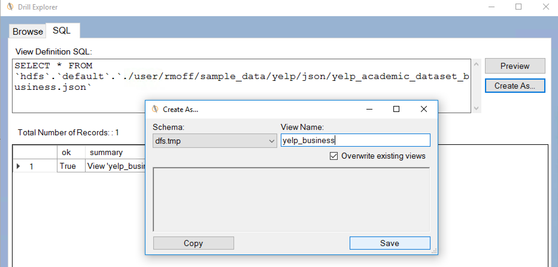
Drill Explorer

The MapR Drill ODBC driver comes with a tool called Drill Explorer. This is a GUI that enables you to explore the data by navigating the databases (==storage plugins) and folders/files within, previewing the data and even creating views on it.

Drill Client

Within the Drill client there are various settings available:

0: jdbc:drill:zk=local> !set  
autocommit          true  
autosave            false  
color               true  
fastconnect         true  
force               false  
headerinterval      100  
historyfile         /home/oracle/.sqlline/history  
incremental         true  
isolation           TRANSACTION_REPEATABLE_READ  
maxcolumnwidth      15  
maxheight           56  
maxwidth            1000000  
numberformat        default  
outputformat        table  
propertiesfile      /home/oracle/.sqlline/sqlline.properties  
rowlimit            0  
showelapsedtime     true  
showheader          true  
shownestederrs      false  
showwarnings        true  
silent              false  
timeout             -1  
trimscripts         true  
verbose             false  

To change one, such as the width of output displayed:

0: jdbc:drill:zk=local> !set maxwidth 10000  

To connect to remote Drill specify the Zookeeper node(s) that store the Drillbit connection information:

rmoff@asgard-3:apache-drill-1.7.0> bin/sqlline -u jdbc:drill:zk=cdh57-01-node-01.moffatt.me:2181,cdh57-01-node-02.moffatt.me:2181,cdh57-01-node-03.moffatt.me:2181  

Conclusion

Apache Drill is a powerful tool for using familiar querying language (SQL) against different data sources. On a small scale, simply being able to slice and dice through structured files like JSON is a massive win. On a larger scale, it will be interesting to experiment with how Apache Drill compares when querying larger volumes of data across a cluster of machines, maybe compared to a tool such as Impala.

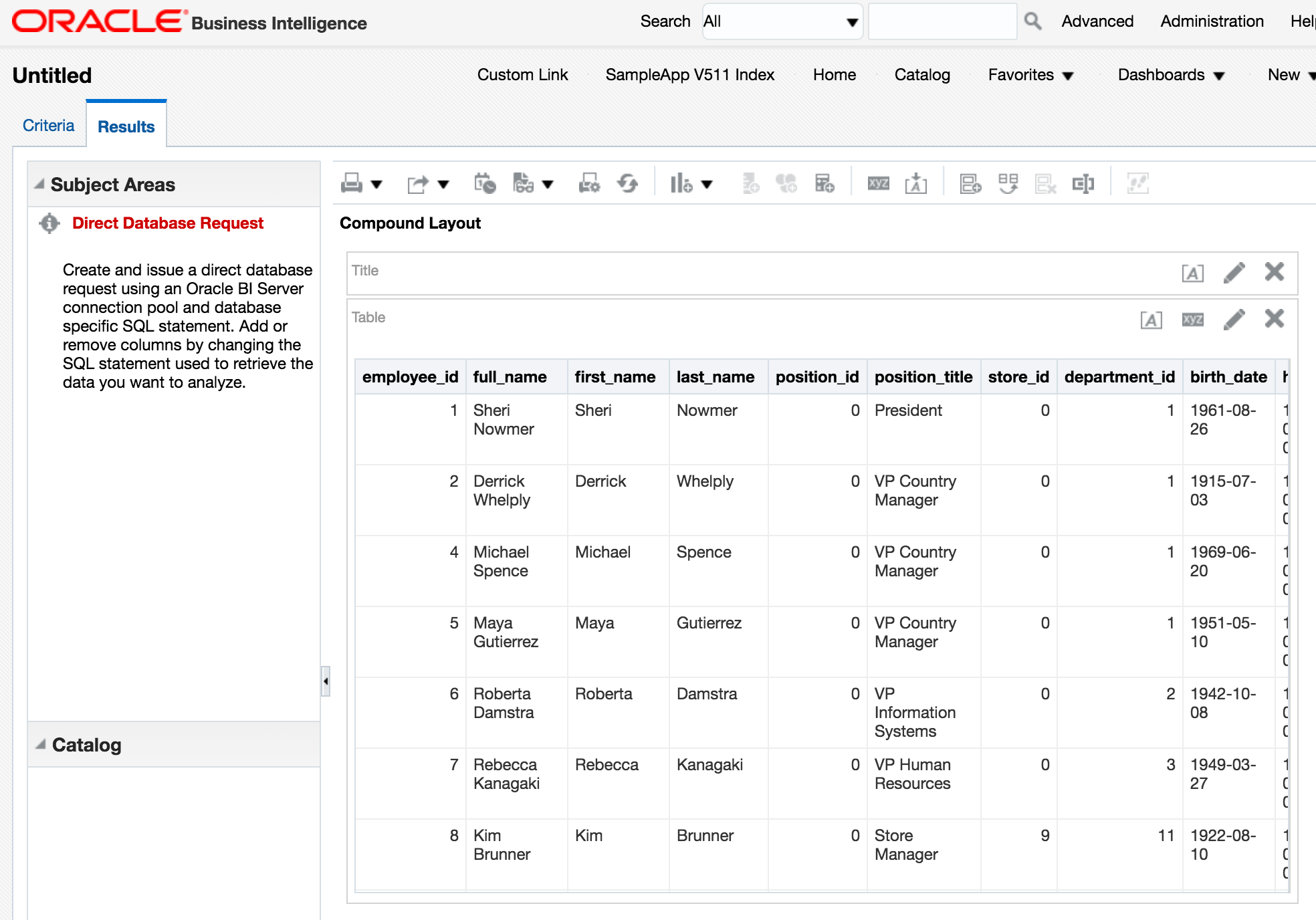
For more information about Apache Drill see how to access Drill from within OBIEE, as well as bonus geeky blog coming soon explaining the debug tools I used to try and figure out why it wouldn't initially work...

Apache Drill enables querying with SQL against a multitude of datasources including things like JSON files, Parquet and Avro, Hive tables, RDBMS and more. MapR have released an ODBC driver for it, and I thought it'd be neat to get it to work with OBIEE. It evidently does work for OBIEE running on Windows, but I wanted to be able to use it on my standard environment, Linux.

For more information on Apache Drill, see my previous post, Introduction to Apache Drill.

OBIEE 12c (and 11g and 10g before it) supports three primary ways of connecting to data sources:

1. Native Gateway, such as OCI for Oracle. This is always the preferred option as it gives the greatest support and performance.
2. Data Direct ODBC Drivers, a set of which are bundled with OBIEE for enabling connectivity to sources such as SQL Server, MySQL, Hive, and Impala. The configuration of these is documented in the OBIEE manuals, and is generally a supported configuration.
3. Native ODBC Drivers.

To get OBIEE to work with Apache Drill we'll use the third option - native ODBC drivers. I'm doing this on SampleApp v511.

First Things First - Setting up Apache Drill

Drill can be deployed in distributed configuration (with all the parallel processing goodness which that brings), but also run as a single instance locally. For the sake of simplicity that's what I'm going to do here. It's rather easy to do:

# Download Apache Drill
wget http://www.apache.org/dyn/closer.cgi/drill/drill-1.7.0/apache-drill-1.7.0.tar.gz
# Unpack
tar -xvf apache-drill-1.7.0.tar.gz
# Run
cd /opt/apache-drill-1.7.0/ && bin/sqlline -u jdbc:drill:zk=local

You need to make sure you've got a recent JDK available, and if you're running it on BigDataLite VM watch out for this odd problem that I had which was related to classpaths and maniested itself with the error java.lang.NoSuchMethodError: com.fasterxml.jackson.databind.JavaType.isReferenceType()Z.

All being well, you'll now have a Drill prompt:

Java HotSpot(TM) 64-Bit Server VM warning: ignoring option MaxPermSize=512M; support was removed in 8.0  
Aug 09, 2016 5:51:43 AM org.glassfish.jersey.server.ApplicationHandler initialize  
INFO: Initiating Jersey application, version Jersey: 2.8 2014-04-29 01:25:26...  
apache drill 1.7.0  
"say hello to my little drill"
0: jdbc:drill:zk=local>  

From here you can run a simple query to check the version:

0: jdbc:drill:zk=local> SELECT version FROM sys.version;  
+----------+
| version  |
+----------+
| 1.7.0    |
+----------+
1 row selected (0.392 seconds)  

or query one of the built-in sample data sets:

0: jdbc:drill:zk=local> select count(*) from cp.`employee.json`;  
+---------+
| EXPR$0  |
+---------+
| 1155    |
+---------+
1 row selected (0.977 seconds)  

For more examples of Drill, see the tutorials.

Setting up Drill ODBC on Linux with OBIEE

With Drill setup and running locally, let's now install the ODBC driver. This is all on SampleApp v511 / Oracle Linux 6.7.

sudo rpm -i http://package.mapr.com/tools/MapR-ODBC/MapR_Drill/MapRDrill_odbc_v1.2.1.1000/MapRDrillODBC-1.2.1.x86_64.rpm

Next, create the MapR Drill ODBC driver configuration file. A sample one is provided, which you can copy from the default installation path of /opt/mapr/drillodbc/Setup/mapr.drillodbc.ini, or create new. I put it in the default path (~/.mapr.drillodbc.ini).

[Driver]
DisableAsync=0  
DriverManagerEncoding=UTF-16  
ErrorMessagesPath=/opt/mapr/drillodbc/ErrorMessages  
LogLevel=2  
LogPath=/tmp/odbc.mapr  
SwapFilePath=/tmp

ODBCInstLib=libodbcinst.so  

In the above I've changed a few things:

• The most important is DriverManagerEncoding. If you leave this as the default of UTF-32 OBIEE will crash (SIGSEGV) when you try to query the data in Apache Drill. You can read all about my trials and tribulations trying to figure this out in a separate blog post coming soon.
• I've set LogLevel to 2 and LogPath to a valid path, so that there's some log files to check if things go wrong
• Set the ODBCInstLib to libodbcinst.so which matches the built in DataDirect ODBC Driver Manager library file.

Following the documentation, Configuring Database Connections Using Native ODBC Drivers:

1. Add the necessary environment variables to BI Server. This is done per-component in a .properties file, which for the BI Server (OBIS / nqsserver) is BI_DOMAIN/config/fmwconfig/bienv/obis/obis.properties, so on SampleApp /app/oracle/biee/user_projects/domains/bi/config/fmwconfig/bienv/OBIS/obis.properties. To this file (which in 12.2.1 is empty by default) we add:

   MAPRDRILLINI=/home/oracle/.mapr.drillodbc.ini
   LD_LIBRARY_PATH=/opt/mapr/drillodbc/lib/64
   

2. Add the Drill DSN to odbc.ini which for OBIEE already exists and is populated with other ODBC configurations. You'll find the file in BI_DOMAIN/config/fmwconfig/bienv/core, which on SampleApp is /app/oracle/biee/user_projects/domains/bi/config/fmwconfig/bienv/core/odbc.ini.

   1. Add to the [ODBC Data Sources] section

      DrillDSN=MapR Drill ODBC Driver 64-bit
      

   2. Add a section to the bottom of the file:

      [DrillDSN]
      Driver=/opt/mapr/drillodbc/lib/64/libmaprdrillodbc64.so
      AuthenticationType=No Authentication
      Description=Drill ODBC Driver
      ConnectionType=Direct
      HOST=localhost
      PORT=31010
      

Now restart the BI Server:

/app/oracle/biee/user_projects/domains/bi/bitools/bin/stop.sh -i obis1 && /app/oracle/biee/user_projects/domains/bi/bitools/bin/start.sh -i obis1

On a Windows machine I installed the MapR Drill ODBC driver too and created a DSN of the same name as in my odbc.ini file above. In the Administration Tool I set up a new Database (type: ODBC Basic) and associated connection pool (ODBC 2.0) pointing to DrillDSN.

Now to try it out! In Answers I build a Direct Database Request:

and run it

Nice. We can query data held in HDFS too, again with a Direct Database Request:

Exploring Drill data with OBIEE

So the above DDR prove the connectivity works. But as any ful kno, DDR is at best a 'tactical' solution, at worst, a complete hack and maintenance nightmare. Let's use the force luke, or at least, the RPD. The first obvious thing to do is Import Metadata from the connection pool that we've defined. But doing this, there's no objects shown:

That's because 'tables' in Drill are not quite as clearly defined as in a standard RDBMS. A table could be a single file, multiple files matching a pattern, or even literally a table if connecting Drill to an RDBMS. So to expose a set of data through Drill, we define a view. This is where Drill Explorer comes in as it gives a simple GUI over the available files

from where you can use the SQL tab and Create As option to create a view

Having done this, launch the Import Metadata dialog again (right click the Connection Pool and select Import Metadata), and make sure you tick Views on the Metadata types to view. Now you'll see the object. Unfortunately, it just has a single column - *. I've not figured out yet how - if if it's possible - to get a view to explode out all columns in the underlying select clause. Import the view:

You'll get an error about the * column name, but the table and schema still get brought across.

Now the slightly tedious bit - define each physical column, and define the physical and logical model, done very simplistically here:

A simple query:

Aaaaaand a simple error:

State: HY000. Code: 16001. [nQSError: 16001] ODBC error state: S1000 code: 1040 message:
[MapR][Drill] (1040) Drill failed to execute the query:
select avg(T29568."stars") as c1, T29568."city" as c2, T29568."full_address" as c3, T29568."name" as c4 from "DRILL"."dfs.tmp"."yelp_business" T29568 group by T29568."city", T29568."full_address", T29568."name" order by 2, 4, 3
[30027]Query execution error. Details:[
PARSE ERROR: Encountered ". \"" at line 1, column 33.
Was expecting one of: ")" ... "ORDER" ... "LIMIT" ... "OFFSET" ... "FETCH" ... "," .... (HY000)

Looking at the query being run, OBIEE is using double quotation marks (") to quote identifiers, but Drill requires backtick (`) instead. Heading over to DB Features can fix this:

And refreshing the report gives:

Conclusion

This is the very basics necessary to get up and running with OBIEE and Apache Drill. It would be good to see if there's an optimal, least-friction, way for getting tables in Drill exposed to OBIEE without needing to enter each physical column.

One of the many powerful features of Drill is being able to access nested and array JSON values, which I've discussed in my Introduction to Apache Drill post. The above examples just use root-level attributes, and could easily be expanded out to process some of the nested fields (such as hours in the business data above). For the time being this would be done with DDR, or a Drill view wrapped around it imported into the Physical layer of the RPD.

OBIEE 12c (and 11g and 10g before it) supports three primary ways of connecting to data sources:

1. Native Gateway, such as OCI for Oracle. This is always the preferred option as it gives the greatest support and performance.
2. Data Direct ODBC Drivers, a set of which are bundled with OBIEE for enabling connectivity to sources such as SQL Server, MySQL, Hive, and Impala. The configuration of these is documented in the OBIEE manuals and is generally a supported configuration.
3. Native ODBC Drivers.

There's also kind of a fourth option, which is JDBC, as explained by Fiston in this excellent post. It's OBIEE 12c only and not fully documented/supported.

In this article we're going to dig into the third option (native ODBC) and look at how it can be used, and also how to troubleshoot it (and the OBIEE stack in general) on Linux.

ODBC (Open Database Connectivity) is a documented API designed to enable applications to work with databases, without one explicitly supporting the other. A comparable protocol is JDBC, which is also widely used (but as yet not fully supported/documented within OBIEE). To use native ODBC drivers with OBIEE on *nix, you install the driver on your OBIEE server and then configure OBIEE to use it. Mark Rittman wrote an example of how to do this with the original Hive ODBC drivers here (before they were formally bundled with OBIEE), and the manual shows how to use it with a native driver for Teradata.

My interest in this is the Apache Drill tool, which enables querying with SQL against a multitude of datasources, including things like JSON files, Hive tables, RDBMS, and more. MapR have released an ODBC driver for it, and I thought it'd be neat to get Apache Drill to work with OBIEE. It evidently does work for OBIEE running on Windows, but I wanted to be able to use it on my standard environment, Linux. This blog post is a warts-and-all exploration of the process I went through to get it to work, since I thought it might be of interest to see some of the forensic methods available when trying to get things to work. For just the headlines, see Using Apache Drill with OBIEE 12c.

First Things First - Setting Up Apache Drill

Drill can be deployed in distributed configuration (with all the parallel processing goodness which that brings), but also run as a single instance locally. For the sake of simplicity that's what I'm going to do here. It's rather easy to do:

# Download Apache Drill
wget http://www.apache.org/dyn/closer.cgi/drill/drill-1.7.0/apache-drill-1.7.0.tar.gz
# Unpack
tar -xvf apache-drill-1.7.0.tar.gz
# Run
cd /opt/apache-drill-1.7.0/ && bin/sqlline -u jdbc:drill:zk=local

You need to make sure you've got a recent JDK available, and if you're running it on SampleApp, watch out for this odd problem that I had which was related to classpaths and manifested itself with the error java.lang.NoSuchMethodError: com.fasterxml.jackson.databind.JavaType.isReferenceType()Z.

All being well, you'll now have a Drill prompt:

Java HotSpot(TM) 64-Bit Server VM warning: ignoring option MaxPermSize=512M; support was removed in 8.0  
Aug 09, 2016 5:51:43 AM org.glassfish.jersey.server.ApplicationHandler initialize  
INFO: Initiating Jersey application, version Jersey: 2.8 2014-04-29 01:25:26...  
apache drill 1.7.0  
"say hello to my little drill"
0: jdbc:drill:zk=local>  

From here you can run a simple query to check the version:

0: jdbc:drill:zk=local> SELECT version FROM sys.version;  
+----------+
| version  |
+----------+
| 1.7.0    |
+----------+
1 row selected (0.392 seconds)  

or query one of the built-in sample data sets:

0: jdbc:drill:zk=local> select count(*) from cp.`employee.json`;  
+---------+
| EXPR$0  |
+---------+
| 1155    |
+---------+
1 row selected (0.977 seconds)  

For more examples of Drill, see the tutorials.

Setting up Drill ODBC on Linux

With Drill setup and running locally, let's now install the ODBC driver. This is all on SampleApp v511 / Oracle Linux 6.7.

sudo rpm -i http://package.mapr.com/tools/MapR-ODBC/MapR_Drill/MapRDrill_odbc_v1.2.1.1000/MapRDrillODBC-1.2.1.x86_64.rpm

Per the system requirements, we need to make sure that we're using one of the supported ODBC Driver Managers, so we'll install iODBC to start with (the other option being unixODBC):

sudo yum install -y unixodbc

Now follow the configuration instructions. To start with we'll do this in isolation of OBIEE to check that it works, and then bring it into OBIEE's world (for example, odbc.ini already exists in OBIEE).

1. Set environment variables

   export ODBCINI=~/.odbc.ini
   export MAPRDRILLINI=~/.mapr.drillodbc.ini
   export LD_LIBRARY_PATH=/opt/mapr/drillodbc/lib/64
   

2. Set up ODBC DSN in ~/.odbc.ini

   [ODBC Data Sources]
   DrillDSN=MapR Drill ODBC Driver 64-bit
   
   
   [DrillDSN]
   Driver=/opt/mapr/drillodbc/lib/64/libmaprdrillodbc64.so
   Description=Drill ODBC Driver
   ConnectionType=Direct
   HOST=localhost
   PORT=31010
   AuthenticationType=No Authentication
   

3. Copy the default ODBC driver manager config

   cp /opt/mapr/drillodbc/Setup/odbcinst.ini ~/.odbcinst.ini
   

4. Configure the Drill ODBC driver in ~/.mapr.drillodbc.ini

   Here I've set the log level to Trace, so that we can see what's going on in depth—in practice this would generate huge amounts of unnecessary log data so set it to a lower value (e.g. 0) for actual use.

   [Driver]
   DisableAsync=0
   DriverManagerEncoding=UTF-32
   ErrorMessagesPath=/opt/mapr/drillodbc/ErrorMessages
   LogLevel=6
   LogPath=/tmp/odbc.log
   SwapFilePath=/tmp
   
   
   ODBCInstLib=libiodbcinst.so.2
   # This is the ODBC Driver Manager library
   # Note the documentation - the DriverManagerEncoding (above) will vary depending
   # on the driver manager in use.
   # See https://drill.apache.org/docs/configuring-odbc-on-linux/#configuring-.mapr.drillodbc.ini
   

Having set this up, we'll now test it:

[oracle@demo ~]$ iodbctest "DSN=DrillDSN"

You should see:

iODBC Demonstration program  
This program shows an interactive SQL processor  
Driver Manager: 03.52.0709.0909  
Driver: 1.2.1.1001 (MapR Drill ODBC Driver)

SQL>  

From where you can enter a command (don't include the ; suffix as this is added automatically)

SQL> SELECT version FROM sys.version

version  
--------
1.7.0

result set 1 returned 1 rows.  

• If you get Unable to locate SQLGetPrivateProfileString function then check that your LD_LIBRARY_PATH includes the location of the Driver Manager (libiodbc.so.2), and that the exact library specified by ODBCInstLib exists—in my installation it was called libiodbcinst.so.2 rather than libiodbc.so as shown in the docs. Also check that you've set MAPRDRILLINI environment variable.
  • libiodbc installs into /usr/lib64 which is one of the default paths checked for library files, hence not including it explicitly in the LD_LIBRARY_PATH environment variable.
• If you just get Have a nice day. with no error but no SQL> prompt, check your ODBC DSN configuration. I hit this issue when inadvertently omitting the AuthenticationType parameter.

If you head over to /tmp/odbc.log/ you should see a file called driver.log with a bunch of trace data in it. Here's the data from the above session, excluding TRACE logs:

Aug 09 06:23:35.701 INFO  1148090112 Driver::LogVersions: SDK Version: 09.05.07.1008  
Aug 09 06:23:35.701 INFO  1148090112 Driver::LogVersions: DSII Version: 1.2.1.1001  
Aug 09 06:23:35.701 INFO  1148090112 Driver::Initialize: Database CHAR Encoding: UTF-8  
Aug 09 06:23:35.701 INFO  1148090112 Driver::Initialize: Database WCHAR Encoding: UTF-8  
Aug 09 06:23:35.701 INFO  1148090112 Driver::Initialize: ANSI CHAR Encoding: UTF-8  
Aug 09 06:23:35.701 INFO  1148090112 Driver::Initialize: Driver Manager WCHAR Encoding: UTF-32LE  
Aug 09 06:23:35.702 INFO  1148090112 Driver::Initialize: Detected Driver Manager: iODBC, 3.52.7  
Aug 09 06:23:35.702 INFO  1148090112 Driver::Initialize: Locale name: en_GB  
Aug 09 06:23:35.702 INFO  1148090112 Driver::Initialize: Bitness: 64-bit  
Aug 09 06:23:35.702 INFO  1148090112 CInterface::SQLAllocHandle: Allocating environment handle.  
Aug 09 06:23:35.702 INFO  1148090112 Environment::SQLSetEnvAttr: Attribute: SQL_ATTR_ODBC_VERSION (200)  
Aug 09 06:23:35.702 INFO  1148090112 EnvironmentAttributes::SetAttribute: Setting ODBC version to: 3  
Aug 09 06:23:35.702 INFO  1148090112 CInterface::SQLAllocHandle: Allocating connection handle.  
Aug 09 06:23:35.702 INFO  1148090112 Connection::SQLSetConnectAttr: Attribute: Unknown Attribute (1051)  
Aug 09 06:23:35.702 INFO  1148090112 ConnectionAttributes::SetAttribute: Invalid attribute: 1051  
Aug 09 06:23:35.704 ERROR 1148090112 Connection::SQLSetConnectAttr: [MapR][ODBC] (10210) Attribute identifier invalid or not supported: 1051  
Aug 09 06:23:35.708 INFO  1148090112 DiracClient::DiracClient: Create a new Dirac Client [194bd90] (handshakeTimeout = 5, queryTimeout = 180)  
Aug 09 06:23:35.708 INFO  1148090112 DiracClient::connect: Connection String 'local=localhost:31010' & Default Schema ''  
Aug 09 06:23:35.712 DEBUG 1148090112 DiracClient::connect: Connection successfully.  
Aug 09 06:23:35.713 INFO  1148090112 Connection::SQLGetInfoW: InfoType: SQL_CURSOR_COMMIT_BEHAVIOR (23)  
Aug 09 06:23:35.713 INFO  1148090112 Connection::SQLGetInfoW: InfoType: SQL_CURSOR_ROLLBACK_BEHAVIOR (24)  
Aug 09 06:23:35.713 INFO  1148090112 Connection::SQLGetInfoW: InfoType: SQL_DRIVER_VER (7)  
Aug 09 06:23:35.713 INFO  1148090112 Connection::SQLGetInfoW: InfoType: SQL_DRIVER_NAME (6)  
Aug 09 06:23:35.713 INFO  1148090112 CInterface::SQLAllocHandle: Allocating statement handle.  
Aug 09 06:23:35.714 INFO  1148090112 Statement::SQLGetStmtAttrW: Attribute: SQL_ATTR_APP_ROW_DESC (10010)  
Aug 09 06:23:35.714 INFO  1148090112 Statement::SQLGetStmtAttrW: Attribute: SQL_ATTR_APP_PARAM_DESC (10011)  
Aug 09 06:23:35.714 INFO  1148090112 Statement::SQLGetStmtAttrW: Attribute: SQL_ATTR_IMP_ROW_DESC (10012)  
Aug 09 06:23:35.714 INFO  1148090112 Statement::SQLGetStmtAttrW: Attribute: SQL_ATTR_IMP_PARAM_DESC (10013)  
Aug 09 06:25:39.409 INFO  1148090112 StatementState::InternalPrepare: Preparing query: SELECT version FROM sys.version  
Aug 09 06:25:39.412 INFO  1148090112 DiracClient::ExecuteStatementDirect: DRResultSet [19494c0] executes query 'SELECT * FROM (SELECT version FROM sys.version) T LIMIT 0'  
Aug 09 06:25:39.412 DEBUG 1148090112 DRResultSet::GetNextRecordBatch: START DEQUEUE. Current ResultQueue Size = 0  
Aug 09 06:25:40.219 DEBUG 979547904 DiracClient::QueryResultsListener: DRResultSet [19494c0]: Handle RecordBatch [34001c40], DrillClientError [0]'  
Aug 09 06:25:40.219 DEBUG 1148090112 DRResultSet::GetNextRecordBatch: END DEQUEUE. Get RecordBatch 34001c40 [m_recordCount = 0 ]. Now ResultQueue Size = 0  
Aug 09 06:25:40.219 DEBUG 1148090112 DRResultSet::InitializeColumns: Column 1 version: {DataMode: OPTIONAL, MinorType: VARCHAR, Precision = 1, Scale = 0}  
Aug 09 06:25:40.219 DEBUG 1148090112 DRResultSet::GetNextRecordBatch: START DEQUEUE. Current ResultQueue Size = 0  
Aug 09 06:25:40.276 DEBUG 979547904 DiracClient::QueryResultsListener: DRResultSet [19494c0]: Handle RecordBatch [0], DrillClientError [0]'  
Aug 09 06:25:40.276 DEBUG 1148090112 DRResultSet::GetNextRecordBatch: status = QRY_COMPLETED.  
Aug 09 06:25:40.276 INFO  1148090112 DiracClient::CloseStatement: Close statement and free query resources  
Aug 09 06:25:40.276 INFO  1148090112 DiracClient::ExecuteStatementDirect: DRResultSet [19494c0] executes query 'SELECT version FROM sys.version'  
Aug 09 06:25:40.277 DEBUG 1148090112 DRResultSet::GetNextRecordBatch: START DEQUEUE. Current ResultQueue Size = 0  
Aug 09 06:25:40.748 DEBUG 979547904 DiracClient::QueryResultsListener: DRResultSet [19494c0]: Handle RecordBatch [3400cb60], DrillClientError [0]'  
Aug 09 06:25:40.750 DEBUG 1148090112 DRResultSet::GetNextRecordBatch: END DEQUEUE. Get RecordBatch 3400cb60 [m_recordCount = 1 ]. Now ResultQueue Size = 0  
Aug 09 06:25:40.750 DEBUG 1148090112 DRResultSet::InitializeColumns: Column 1 version: {DataMode: OPTIONAL, MinorType: VARCHAR, Precision = 1, Scale = 0}  
Aug 09 06:25:40.751 DEBUG 1148090112 DRResultSet::GetNextRecordBatch: START DEQUEUE. Current ResultQueue Size = 0  
Aug 09 06:25:40.985 DEBUG 979547904 DiracClient::QueryResultsListener: DRResultSet [19494c0]: Handle RecordBatch [0], DrillClientError [0]'  
Aug 09 06:25:40.985 DEBUG 1148090112 DRResultSet::GetNextRecordBatch: status = QRY_COMPLETED.  
Aug 09 06:25:40.986 INFO  1148090112 DiracClient::CloseStatement: Close statement and free query resources  
Aug 09 06:25:40.991 ERROR 1148090112 Statement::SQLCloseCursor: [MapR][ODBC] (10510) Invalid cursor state.  
Aug 09 06:27:19.748 ERROR 1148090112 Statement::SQLCloseCursor: [MapR][ODBC] (10510) Invalid cursor state.  
Aug 09 06:27:19.748 INFO  1148090112 CInterface::SQLFreeHandle: Freeing statement handle.  
Aug 09 06:27:19.748 INFO  1148090112 DiracClient::~DiracClient: Close the Dirac Client [194bd90]  
Aug 09 06:27:19.748 INFO  1148090112 CInterface::SQLFreeHandle: Freeing connection handle.  
Aug 09 06:27:19.749 INFO  1148090112 CInterface::SQLFreeHandle: Freeing environment handle.  

Hooking it up to OBIEE

We've shown that we can connect to Apache Drill using ODBC and query it. Let's see if we get it to work for OBIEE. Our starting point is the 12c docs, Configuring Database Connections Using Native ODBC Drivers.

1. Environment variables are defined per-component in a .properties file, which for the BI Server (OBIS / nqsserver) is BI_DOMAIN/config/fmwconfig/bienv/obis/obis.properties, so on SampleApp /app/oracle/biee/user_projects/domains/bi/config/fmwconfig/bienv/OBIS/obis.properties. To this file (which in 12.2.1 is empty by default) we add:

   MAPRDRILLINI=/home/oracle/.mapr.drillodbc.ini
   LD_LIBRARY_PATH=/opt/mapr/drillodbc/lib/64
   

2. Add the Drill DSN to odbc.ini which for OBIEE already exists and is populated with other ODBC configurations. You'll find the file in BI_DOMAIN/config/fmwconfig/bienv/core, which on SampleApp is /app/oracle/biee/user_projects/domains/bi/config/fmwconfig/bienv/core/odbc.ini.

   1. Add to the [ODBC Data Sources] section

      DrillDSN=MapR Drill ODBC Driver 64-bit
      

   2. Add a section to the bottom of the file:

      [DrillDSN]
      Driver=/opt/mapr/drillodbc/lib/64/libmaprdrillodbc64.so
      AuthenticationType=No Authentication
      Description=Drill ODBC Driver
      ConnectionType=Direct
      HOST=localhost
      PORT=31010
      

Now restart the BI Server:

/app/oracle/biee/user_projects/domains/bi/bitools/bin/stop.sh -i obis1 && /app/oracle/biee/user_projects/domains/bi/bitools/bin/start.sh -i obis1

We can check that the BI Server has picked up our new environment variables by using the /proc pseudo file-system (you can also see an environment variable dump as part of the obis1.out logfile during startup):

[oracle@demo ~]$ strings /proc/$(pgrep nqsserver)/environ|grep mapr
LD_LIBRARY_PATH=/app/oracle/biee/bi/common/ODBC/Merant/7.1.4/lib:/app/oracle/biee/bi/bifoundation/server/bin:/app/oracle/biee/bi/bifoundation/web/bin:/app/oracle/biee/bi/clients/Essbase/EssbaseRTC/bin:/app/oracle/biee/bi/lib:/app/oracle/biee/lib:/app/oracle/biee/oracle_common/adr:/app/oracle/biee/oracle_common/lib:/usr/lib:/lib:/opt/mapr/drillodbc/lib/64:::/app/oracle/app/oracle/product/12.1.0/dbhome_1/lib:/app/oracle/endeca/olt/bin:/app/oracle/biee/wlserver/server/native/linux/x86_64:/app/oracle/biee/wlserver/server/native/linux/x86_64/oci920_8:/app/oracle/biee/wlserver/server/native/linux/x86_64:/app/oracle/biee/wlserver/server/native/linux/x86_64/oci920_8
MAPRDRILLINI=/home/oracle/.mapr.drillodbc.ini

Over in the Administration Tool I set up a new Database (type: ODBC Basic) and associated connection pool (ODBC 2.0) pointing to DrillDSN.

Now to try it out! In Answers I build a Direct Database Request:

But...oh no!

Odbc driver returned an error (SQLExecDirectW).
State: HY000. Code: 10058. [NQODBC] [SQL_STATE: HY000] [nQSError: 10058] A general error has occurred. (HY000)
State: HY000. Code: 12010. [nQSError: 12010] Communication error connecting to remote end point: address = demo.us.oracle.com; port = 7792. (HY000)
SQL Issued: {call NQSGetQueryColumnInfo('EXECUTE PHYSICAL CONNECTION POOL "Apache Drill"."Apache Drill" SELECT version FROM sys.version;')}

Let's pick through this, because it's a common error and easily misinterpreted.

1. Odbc driver returned an error (SQLExecDirectW).

   • When you run an analysis/dashboard, Presentation Services (OBIPS/sawserver) connects to the BI Server (OBIS/nqsserver) to send the request as Logical SQL, and it connects to the BI Server using ODBC. Therefore any kind of issue running the request will always show as an "ODBC error".

   • Learning: nothing, other than that Presentation Services hit an error.

2. State: HY000. Code: 10058. [NQODBC] [SQL_STATE: HY000] [nQSError: 10058] A general error has occurred. (HY000)

   • Learning: nothing. Something went wrong, somewhere, and OBIEE was involved (nQSError).

3. State: HY000. Code: 12010. [nQSError: 12010] Communication error connecting to remote end point: address = demo.us.oracle.com; port = 7792. (HY000)

   • Now we're getting somewhere. Port 7792 is, on this server, the BI Server (OBIS / nqsserver). And, there was an error connecting to it.
   • Learning: We failed to successfully connect to the BI Server. Is it running? Was it running but crashed? Is there a network problem? Lots to investigate.

4. SQL Issued: {call NQSGetQueryColumnInfo('EXECUTE PHYSICAL CONNECTION POOL "Apache Drill"."Apache Drill" SELECT version FROM sys.version;')}

   • Learning: This is the logical SQL that Presentation Services was trying to run. Useful to know.

Let's go and have a look at the BI Server log, because something's evidently not right. We know that it was running, because otherwise we'd not have been able to login to OBIEE in the first place.

In /app/oracle/biee/user_projects/domains/bi/servers/obis1/logs/obis1.out there's some bad news:

<NodeManager ComponentManager> <The server 'obis1' with process id 7059 is no longer alive; waiting for the process to die.>
<NodeManager ComponentManager> <Process died.>
<NodeManager ComponentManager> <get latest startup configuration before deciding/trying to restart the server>
<NodeManager ComponentManager> <Server failed so attempting to restart (restart count = 1)>

So it looks like the BI Server crashed. In the folder above where obis1.out is kept, there's a corresponding crash report (note that the process ID matches the log message above), nqsserver_7059_crashreport.txt. Some bits of interest from it:

[...]
Beginning of crash dump...  
Signal: 11  
================================================================
[...]
Activity type: ExecutePhysical GatewayDbGateway Prepare  
DSN:Apache Drill  
User Name:weblogic  
SQL:SELECT version FROM sys.version;  
================================================================
Activity #2 ECID: 005EPt5qYm2Fw000jzwkno0001iJ0001KT,0  
================================================================
Activity type: Producer Executing Query  
Repository Name:ssi;Subject Area Name:;User Name:weblogic  
Logical Hash of SQL: 0x3d5c4ef2SQL:{call NQSGetQueryColumnInfo('EXECUTE PHYSICAL  CONNECTION POOL "Apache Drill"."Apache Drill" SELECT version FROM sys.version;')}  
[...]

BACKTRACE:  
/app/oracle/biee/bi/bifoundation/server/bin/libnqutilityserver64.so(+0x12a829)[0x7f554995b829]
/lib64/libpthread.so.0(+0xf790)[0x7f5547cde790]
/lib64/libc.so.6(cfree+0x1c)[0x7f554721693c]
/app/oracle/biee/bi/common/ODBC/Merant/7.1.4/lib/libodbc.so(+0xa5c55)[0x7f550f2efc55]
/app/oracle/biee/bi/common/ODBC/Merant/7.1.4/lib/libodbc.so(+0xa4fc0)[0x7f550f2eefc0]
/app/oracle/biee/bi/common/ODBC/Merant/7.1.4/lib/libodbc.so(+0xa53f0)[0x7f550f2ef3f0]
/app/oracle/biee/bi/common/ODBC/Merant/7.1.4/lib/libodbc.so(SQLDriverConnect+0x149)[0x7f550f2d8337]
/app/oracle/biee/bi/bifoundation/server/bin/libnqsdbgatewayodbc64.so(_ZN8NQSQLAPI18NQSQLDriverConnectEPvS0_RKN3sup6StringIwN7_SASSTL9allocatorIwEEEES8_S8_tbS8_+0x1c8)[0x7f54abfb5078]
/app/oracle/biee/bi/bifoundation/server/bin/libnqsdbgatewayodbc64.so(_ZN24OdbcDataSourceConnection7ConnectERK6SignonbjN10ServerInfo17TxnIsolationLevelEi+0x275)[0x7f54abfcbb45]
/app/oracle/biee/bi/bifoundation/server/bin/libnqutilityserver64.so(_ZN20DataSourceConnection7ConnectERK6SignonbRK14GatewayOptions+0x79)[0x7f55498d6819]
/app/oracle/biee/bi/bifoundation/server/bin/libnqsdbconnection64.so(_ZN12DbConnection9FixDamageERK14GatewayOptions+0x7c)[0x7f55524e12cc]
/app/oracle/biee/bi/bifoundation/server/bin/libnqsdbconnection64.so(_ZN20SingleThreadedDbPool22GetAvailableConnectionERK6SignonR17DbConnectionGuardRbRK14GatewayOptions+0x45e)[0x7f555250513e]
/app/oracle/biee/bi/bifoundation/server/bin/libnqsdbgateway64.so(_ZN11NQDbGateway7PrepareEv+0xb14)[0x7f5552294fa4]
/app/oracle/biee/bi/bifoundation/server/bin/libnqsexecutionlist64.so(_ZN8Producer11ExecuteOnceEv+0xb4c)[0x7f555146192c]
/app/oracle/biee/bi/bifoundation/server/bin/libnqutilitygeneric64.so(_ZN16NQExecutionState17ExecuteSystemMainEv+0x82)[0x7f5549c92032]
/app/oracle/biee/bi/bifoundation/server/bin/libnqutilitygeneric64.so(_ZN15NQThreadJobBase17ExecuteSystemMainEv+0x51)[0x7f5549cd9dd1]
/app/oracle/biee/bi/bifoundation/server/bin/libnqsdbconnection64.so(_ZN18NQThreadServerBaseI17ManagedJobFunctorE11ScheduleJobEv+0x40)[0x7f5552509650]
/app/oracle/biee/bi/bifoundation/server/bin/libnqutilitygeneric64.so(_ZN19NQThreadServerNoJob15ExecuteUserMainEv+0x16)[0x7f5549cda256]
/app/oracle/biee/bi/bifoundation/server/bin/libnqutilitygeneric64.so(_ZN16NQExecutionState17ExecuteSystemMainEv+0x82)[0x7f5549c92032]
/app/oracle/biee/bi/bifoundation/server/bin/libnqutilitygeneric64.so(_ZN8NQThread17ExecuteSystemMainEv+0x5b)[0x7f5549cd897b]
/app/oracle/biee/bi/bifoundation/server/bin/libnqutilitygeneric64.so(_ZN8NQThread15ThreadMainEntryEPv+0x2e)[0x7f5549cd8c9e]
/lib64/libpthread.so.0(+0x7a51)[0x7f5547cd6a51]
/lib64/libc.so.6(clone+0x6d)[0x7f554728393d]

Signal 11 is "SIGSEGV", or segmentation fault, which is bad, m'kay?

Tracing OBIEE's ODBC Connectivity with strace

Looking in at the ODBC driver.log we can see that something happened, but no error logged. Here's everything, minus TRACE logs:

Aug 09 07:13:43.283 INFO  2896611072 Driver::LogVersions: SDK Version: 09.05.07.1008  
Aug 09 07:13:43.288 INFO  2896611072 Driver::LogVersions: DSII Version: 1.2.1.1001  
Aug 09 07:13:43.288 INFO  2896611072 Driver::Initialize: Database CHAR Encoding: UTF-8  
Aug 09 07:13:43.288 INFO  2896611072 Driver::Initialize: Database WCHAR Encoding: UTF-8  
Aug 09 07:13:43.288 INFO  2896611072 Driver::Initialize: ANSI CHAR Encoding: UTF-8  
Aug 09 07:13:43.288 INFO  2896611072 Driver::Initialize: Driver Manager WCHAR Encoding: UTF-32LE  
Aug 09 07:13:43.289 INFO  2896611072 Driver::Initialize: Detected Driver Manager: DataDirect Driver Manager, 07.14.0119 (U0115)  
Aug 09 07:13:43.289 INFO  2896611072 Driver::Initialize: Locale name: en_US  
Aug 09 07:13:43.289 INFO  2896611072 Driver::Initialize: Bitness: 64-bit  
Aug 09 07:13:43.290 INFO  2896611072 CInterface::SQLAllocHandle: Allocating environment handle.  
Aug 09 07:13:43.293 INFO  2896611072 CInterface::SQLAllocHandle: Allocating connection handle.  
Aug 09 07:13:43.298 ERROR 2896611072 CInterface::SQLGetConnectAttr: [MapR][ODBC] (10210) Attribute identifier invalid or not supported: 1063  
Aug 09 07:13:43.300 INFO  2896611072 CInterface::SQLFreeHandle: Freeing connection handle.  
Aug 09 07:13:43.301 INFO  2896611072 CInterface::SQLFreeHandle: Freeing environment handle.  
Aug 09 07:13:43.312 INFO  2896611072 CInterface::SQLAllocHandle: Allocating environment handle.  
Aug 09 07:13:43.315 INFO  2896611072 Environment::SQLSetEnvAttr: Attribute: SQL_ATTR_ODBC_VERSION (200)  
Aug 09 07:13:43.315 INFO  2896611072 EnvironmentAttributes::SetAttribute: Setting ODBC version to: 2  
Aug 09 07:13:43.315 INFO  2896611072 CInterface::SQLAllocHandle: Allocating connection handle.  
Aug 09 07:13:43.317 INFO  2896611072 Environment::SQLGetEnvAttr: Attribute: Unknown Attribute (1065)  
Aug 09 07:13:43.317 INFO  2896611072 Connection::SQLGetInfoW: InfoType: SQL_DRIVER_ODBC_VER (77)  

One thing that stands out (with the benefit of hindsight because I've been hacking away at this for a while) is

Driver::Initialize: Detected Driver Manager: DataDirect Driver Manager, 07.14.0119 (U0115)

Whereas in my successful standalone test above it was

Driver::Initialize: Detected Driver Manager: iODBC, 3.52.7

So now let's do some digging. Using strace (which I've written about previously) we can see every system call that OBIEE makes, letting us audit the files that it reads and libraries that it loads. You can invoke strace at process startup or, easier, attach it to a running one. Since the BI Server also creates child processes, and also may crash (as here), we'll use a loop to make sure we've always got a strace running against it until we opt to cancel it:

while [ 1 -eq 1 ]; do strace -f -p $(pgrep nqsserver) -tt -y -s 4096 -o ~/nqs_trace_$(date +%Y%m%dT%H%M%S%N).out;done

If the BI Server isn't running, you'll just see

strace: Invalid process id: '-tt'

But once it starts, you'll get

Process 8457 attached

The output is written to the home folder, in files named nqs_trace_ followed by the timestamp at which the trace started. To cancel it, hit Ctrl-C several times to break out of strace and the while loop. If you leave this running for a long period of time you'll likely fill the filesystem and possibly make the server unusable…

Using your text editor of choice, you can search through the strace output to try and pick apart what's happening. Even if you don't find the cause of the error, you can at least rule other causes out this way. For example, whether a configuration file that you think is being used actually is, or where a library is actually being read from.

First up in searching the trace for odbc is the BI Server's own ODBC gateway library being opened and read:

7222  07:13:43.080212 open("/app/oracle/biee/bi/bifoundation/server/bin/libnqsdbgatewayodbc64.so", O_RDONLY) = 31

Next it checks for the odbc.ini configuration file and gets a success return code (0), but at this point it doesn't read it

8382  07:13:43.097901 stat("/app/oracle/biee/user_projects/domains/bi/config/fmwconfig/bienv/core/odbc.ini", {st_mode=S_IFREG|0640, st_size=2613, ...}) = 0

and then looks for the ODBC trace library, and this is interesting because it can't find it. One of the very useful things with strace is to be able to see all the paths that a program tries to read for a given file. Here you see a selection of the paths it's trying, and the failure (-1 ENOENT (No such file or directory)) each time:

8382  07:13:43.098135 stat("/app/oracle/biee/bi/common/ODBC/Merant/7.1.4/lib/odbctrac.so", 0x7f54aca68b90) = -1 ENOENT (No such file or directory)
8382  07:13:43.098190 stat("/usr/local/lib//app/oracle/biee/bi/common/ODBC/Merant/7.1.4/lib/odbctrac.so", 0x7f54aca68b90) = -1 ENOENT (No such file or directory)
8382  07:13:43.098230 stat("/usr/local/lib/..//app/oracle/biee/bi/common/ODBC/Merant/7.1.4/lib/odbctrac.so", 0x7f54aca68b90) = -1 ENOENT (No such file or directory)
8382  07:13:43.098274 stat("/app/oracle/biee/bi/common/ODBC/Merant/7.1.4/lib//app/oracle/biee/bi/common/ODBC/Merant/7.1.4/lib/odbctrac.so", 0x7f54aca68b90) = -1 ENOENT (No such file or directory)
8382  07:13:43.098312 stat("/app/oracle/biee/bi/common/ODBC/Merant/7.1.4/lib/..//app/oracle/biee/bi/common/ODBC/Merant/7.1.4/lib/odbctrac.so", 0x7f54aca68b90) = -1 ENOENT (No such file or directory)

We can use one of my favourite linux utilities, locate, to find where this file actually is:

[oracle@demo ~]$ locate odbctrac.so
/app/oracle/biee/bi/bifoundation/odbc/lib/odbctrac.so
/app/oracle/biee/bi/common/ODBC/Merant/5.3/lib/odbctrac.so

You can install this on your system with sudo yum install -y mlocate, and if you've recently changed files (e.g. installed a new package) refresh the database with sudo updatedb before running locate.

This is one interesting point of note here, then, that the ODBC trace library isn't loading properly. Let's note this for now, and carry on through the trace file. Next up it opens and reads the odbc.ini file:

8382  07:13:43.102664 open("/app/oracle/biee/user_projects/domains/bi/config/fmwconfig/bienv/core/odbc.ini", O_RDONLY) = 31
8382  07:13:43.102786 read(31</app/oracle/biee/user_projects/domains/bi/config/fmwconfig/bienv/core/odbc.ini>, "[ODBC]\nTrace=1\nTraceFile=/app/oracle/biee/user_projects/domains/bi/odbctrace.out\nTraceDll=/app/oracle/biee/bi/common/ODBC/M [...]

Now we get into the meat of it. The Apache Drill ODBC driver gets checked that it exists:

8382  07:13:43.109475 stat("/opt/mapr/drillodbc/lib/64/libmaprdrillodbc64.so", {st_mode=S_IFREG|0645, st_size=38794216, ...}) = 0

and then opened and read. Next OBIEE tries to read the libdrillClient.so library, starting here:

8382  07:13:43.113071 open("/app/oracle/biee/bi/common/ODBC/Merant/7.1.4/lib/libdrillClient.so", O_RDONLY) = -1 ENOENT (No such file or directory)

Note that this fails (-1 ENOENT), and it works it's way through other paths until it succeeds:

8382  07:13:43.113071 open("/app/oracle/biee/bi/common/ODBC/Merant/7.1.4/lib/libdrillClient.so", O_RDONLY) = -1 ENOENT (No such file or directory)
8382  07:13:43.113189 open("/app/oracle/biee/bi/bifoundation/server/bin/libdrillClient.so", O_RDONLY) = -1 ENOENT (No such file or directory)
8382  07:13:43.113238 open("/app/oracle/biee/bi/bifoundation/web/bin/libdrillClient.so", O_RDONLY) = -1 ENOENT (No such file or directory)
8382  07:13:43.113274 open("/app/oracle/biee/bi/clients/Essbase/EssbaseRTC/bin/libdrillClient.so", O_RDONLY) = -1 ENOENT (No such file or directory)
8382  07:13:43.113309 open("/app/oracle/biee/bi/lib/libdrillClient.so", O_RDONLY) = -1 ENOENT (No such file or directory)
8382  07:13:43.113341 open("/app/oracle/biee/lib/libdrillClient.so", O_RDONLY) = -1 ENOENT (No such file or directory)
8382  07:13:43.113374 open("/app/oracle/biee/oracle_common/adr/libdrillClient.so", O_RDONLY) = -1 ENOENT (No such file or directory)
8382  07:13:43.113408 open("/app/oracle/biee/oracle_common/lib/libdrillClient.so", O_RDONLY) = -1 ENOENT (No such file or directory)
8382  07:13:43.113440 open("/usr/lib/libdrillClient.so", O_RDONLY) = -1 ENOENT (No such file or directory)
8382  07:13:43.113484 open("/lib/libdrillClient.so", O_RDONLY) = -1 ENOENT (No such file or directory)
8382  07:13:43.113517 open("/opt/mapr/drillodbc/lib/64/libdrillClient.so", O_RDONLY) = 31

Where do these paths come from? LD_LIBRARY_PATH! And we can confirm that by comparing the above sequence of folders with the value of LD_LIBRARY_PATH that we saw above, split out onto lines here with a bit of sed magic:

[oracle@demo ~]$  strings /proc/$(pgrep nqsserver)/environ|grep LD_LIBRARY_PATH|sed 's/:/\n/g'|sed 's/=/\n/g'
LD_LIBRARY_PATH
/app/oracle/biee/bi/common/ODBC/Merant/7.1.4/lib
/app/oracle/biee/bi/bifoundation/server/bin
/app/oracle/biee/bi/bifoundation/web/bin
/app/oracle/biee/bi/clients/Essbase/EssbaseRTC/bin
/app/oracle/biee/bi/lib
/app/oracle/biee/lib
/app/oracle/biee/oracle_common/adr
/app/oracle/biee/oracle_common/lib
/usr/lib
/lib
/opt/mapr/drillodbc/lib/64

So...we've read the odbc.ini config file, loaded the Apache Drill ODBC driver (libmaprdrillodbc64.so) and associated library (libdrillClient.so). Now a further library is opened and read:

8382  07:13:43.271710 open("/opt/mapr/drillodbc/lib/64/SimbaDrillODBC.did", O_RDONLY) = 31

and then the Apache Drill ODBC driver configuration file that we created earlier (and referenced in the MAPRDRILLINI environment variable) is opened and read:

8382  07:13:43.281356 open("/home/oracle/.mapr.drillodbc.ini", O_RDONLY) = 31

Because we've enabled logging in the driver configuration, what happens next in the strace is that log file being created and written to:

8382  07:13:43.283527 mkdir("/tmp/odbc.log/", 0755) = -1 EEXIST (File exists)
8382  07:13:43.283834 open("/tmp/odbc.log/driver.log", O_WRONLY|O_CREAT|O_APPEND, 0666) = 31
8382  07:13:43.284037 fstat(31</tmp/odbc.log/driver.log>, {st_mode=S_IFREG|0640, st_size=174018, ...}) = 0
8382  07:13:43.284220 mmap(NULL, 4096, PROT_READ|PROT_WRITE, MAP_PRIVATE|MAP_ANONYMOUS, -1, 0) = 0x7f54ad460000
8382  07:13:43.284338 fstat(31</tmp/odbc.log/driver.log>, {st_mode=S_IFREG|0640, st_size=174018, ...}) = 0
8382  07:13:43.284389 lseek(31</tmp/odbc.log/driver.log>, 174018, SEEK_SET) = 174018
8382  07:13:43.284438 write(31</tmp/odbc.log/driver.log>, "Aug 09 07:13:43.283 INFO  2896611072 Driver::LogVersions: SDK Version: 09.05.07.1008\n", 85) = 85
[...]

After a bunch of trace logging is written, the ODBC messages translation file is read:

8382  07:13:43.290888 read(34</opt/mapr/drillodbc/ErrorMessages/en-US/ODBCMessages.xml>, "<?xml version=\"1.0\" encoding=\"utf-8\"?>\n<!DOCTYPE Messages [\n    <!ELEMENT Messages (Package*)>\n\n    <!ELEMENT Package (Error*)>\n    <!ATTLI

The next file read is odbc.ini again

8382  07:13:43.304659 read(35</app/oracle/biee/user_projects/domains/bi/config/fmwconfig/bienv/core/odbc.ini>, "", 4096) = 0

followed by odbc.ini in the default /etc/ path (which exists but is zero bytes):

8382  07:13:43.306727 open("/etc/odbc.ini", O_RDONLY) = 35

The odbcinst.ini file is then read, from /etc/odbcinst.ini (which is created by unixODBC on installation, and has entries for non-existant mysql/postgresql drivers):

8382  07:13:43.307417 read(35</etc/odbcinst.ini>, "# Example driver definitions\n\n# Driver from the postgresql-odbc package\n# Setup from the unixODBC package\n[PostgreSQL]\nDescription\t= ODBC for PostgreSQL\nDriver\t\t= /usr/lib/psqlod

and then the version for Drill:

8382  07:13:43.308040 read(35</home/oracle/.odbcinst.ini>, "[ODBC Drivers]\nMapR Drill ODBC Driver 64-bit=Installed\n\n[MapR Drill ODBC Driver 64-bit]\nDescription=MapR Drill ODBC Driver(64-bit)\nDriver=/opt/mapr/drillodbc/lib/64/libmaprd

Back to the odbc.ini file, both OBIEE and default (empty) system:

8382  07:13:43.309065 open("/app/oracle/biee/user_projects/domains/bi/config/fmwconfig/bienv/core/odbc.ini", O_RDONLY) = 35
8382  07:13:43.309619 read(35</etc/odbc.ini>, "", 4096) = 0

After another read of the two odbcinst.ini files (per above), there's logging information written

8382  07:13:43.312345 write(31</tmp/odbc.log/driver.log>, "Aug 09 07:13:43.312 INFO  2896611072 CInterface::SQLAllocHandle: Allocating environment handle.\n", 96) = 96
[...]
8382  07:13:43.317106 write(31</tmp/odbc.log/driver.log>, "Aug 09 07:13:43.317 INFO  2896611072 Connection::SQLGetInfoW: InfoType: SQL_DRIVER_ODBC_VER (77)\n", 97) = 97
8382  07:13:43.317141 stat("/tmp/odbc.log/driver.log", {st_mode=S_IFREG|0640, st_size=179550, ...}) = 0

And then, bang.

8382  07:13:43.317198 --- SIGSEGV {si_signo=SIGSEGV, si_code=SEGV_MAPERR, si_addr=0x1f} ---

After which, the crashreport is written:

8382  07:13:43.317249 open("/app/oracle/biee/user_projects/domains/bi/servers/obis1/nqsserver_7059_crashreport.txt", O_WRONLY|O_CREAT|O_APPEND, 0600) = 35
[...]

So from this we can see that the ODBC driver is being loaded from the path we expected, and the configuration files that we expected are being read too. So no smoking gun - but a couple of possible problems ruled out.

Reproducing the Crash on Demand

With this kind of problem it's often a case of working through lots of different configuration settings to obtain further diagnostic evidence - which requires reproducing the problem each time. Instead of manually running the query through Answers which triggers the problem, I moved this part of the diagnostics to the command line, with nqcmd. I copied the logical SQL to a file drill-test.lsql:

EXECUTE PHYSICAL CONNECTION POOL "Apache Drill"."Apache Drill" SELECT version FROM sys.version;

and then run with:

/app/oracle/biee/user_projects/domains/bi/bitools/bin/nqcmd.sh -d AnalyticsWeb -u weblogic -p Admin123 -s ~/drill-test.lsql

gives the same result (error) but easier to do.

Aug 09, 2016 7:59:53 PM oracle.bi.endpointmanager.impl.bienv.BIEnvComponents loadFromInputStream  
INFO: Reading components from: /app/oracle/biee/user_projects/domains/bi/config/fmwconfig/bienv/core/bienv-components.xml ...

-------------------------------------------------------------------------------
          Oracle BI ODBC Client
          Copyright (c) 1997-2015 Oracle Corporation, All rights reserved
-------------------------------------------------------------------------------


EXECUTE PHYSICAL CONNECTION POOL "Apache Drill"."Apache Drill" SELECT version FROM sys.version  
EXECUTE PHYSICAL CONNECTION POOL "Apache Drill"."Apache Drill" SELECT version FROM sys.version  
[unixODBC][nQSError: 12010] Communication error connecting to remote end point: address = demo.us.oracle.com; port = 7792.[unixODBC][NQODBC] [SQL_STATE: S1000] [nQSError: 10058] A general error has occurred.

Statement preparation failed


Processed: 1 queries  
Encountered 1  errors  

Stuff Ruled Out

• The odbcinst.ini file doesn't have to be present - strace showed it is looked for, but the result is the same even if it's not (or is but doesn't have an entry for the Drill drivers):

  4270  20:00:06.692891 open("/home/oracle/.odbcinst.ini", O_RDONLY) = -1 ENOENT (No such file or directory)
  

• Changing the connection pool call interface to ODBC 3.5 doesn't fix things, nor does changing the database type to Apache Hadoop (grasping at straws...)

Driver Manager

One of the routes of investigation is the Driver Manager. This is for two reasons; one is that on Windows ODBC is native, the driver manager is built in. As mentioned, @cfiston has got this to work - but on Windows. So platform differences aside (he says casually), this could be something. The second reason is the difference in the driver manager that shows in the ODBC log between a successful (via iodbctest) request

Driver::Initialize: Detected Driver Manager: iODBC, 3.52.7

versus an unsuccessful one (in OBIEE):

Driver::Initialize: Detected Driver Manager: DataDirect Driver Manager, 07.14.0119 (U0115)

Before we dig into this further let's take a look at the driver manager libraries that we've got on the system. DataDirect and unixODBC are both libodbcinst.so whilst iODBC is libiodbc.so. We'll use a bit of bash magic to find all the files, and list their sizes and checksums so we can spot which are the same:

[oracle@demo odbc.log]$ locate libodbcinst|xargs -Ifoo ls -l foo
-rw-r----- 1 oracle oinstall 1380087 2015-10-13 03:04 /app/oracle/biee/bi/bifoundation/odbc/lib/libodbcinst.so
-rw-r----- 1 oracle oinstall 1380087 2015-10-03 02:59 /app/oracle/biee/bi/common/ODBC/Merant/5.3/lib/libodbcinst.so
-rw-r----- 1 oracle oinstall 1203032 2015-10-03 02:59 /app/oracle/biee/bi/common/ODBC/Merant/7.0.1/lib/libodbcinst.so
-rw-r----- 1 oracle oinstall 1239728 2015-10-03 02:59 /app/oracle/biee/bi/common/ODBC/Merant/7.1.2/lib/libodbcinst.so
-rw-r----- 1 oracle oinstall 1244304 2015-10-03 02:59 /app/oracle/biee/bi/common/ODBC/Merant/7.1.4/lib/libodbcinst.so
lrwxrwxrwx 1 root root 20 2016-08-08 11:55 /usr/lib64/libodbcinst.so -> libodbcinst.so.2.0.0  
lrwxrwxrwx 1 root root 20 2016-08-08 11:55 /usr/lib64/libodbcinst.so.2 -> libodbcinst.so.2.0.0  
-rwxr-xr-x 1 root root 68928 2014-08-16 19:58 /usr/lib64/libodbcinst.so.2.0.0

[oracle@demo odbc.log]$ locate libodbcinst|xargs -Ifoo md5sum foo|sort
0bfd147ff6b41daee527861143040f1b  /app/oracle/biee/bi/common/ODBC/Merant/7.1.2/lib/libodbcinst.so  
7eaee346f92169fc2e2ba5900dceefa3  /app/oracle/biee/bi/common/ODBC/Merant/5.3/lib/libodbcinst.so  
b340968ee0a2188427a66203fb0a56b7  /app/oracle/biee/bi/bifoundation/odbc/lib/libodbcinst.so  
dadcb67d26d42b0c2535a9be44d2b46f  /usr/lib64/libodbcinst.so  
dadcb67d26d42b0c2535a9be44d2b46f  /usr/lib64/libodbcinst.so.2  
dadcb67d26d42b0c2535a9be44d2b46f  /usr/lib64/libodbcinst.so.2.0.0  
eccb81df3cdaaeb83faa86dfc6187844  /app/oracle/biee/bi/common/ODBC/Merant/7.1.4/lib/libodbcinst.so  
ed27493fd52534e181e0e6cd29c6a48a  /app/oracle/biee/bi/common/ODBC/Merant/7.0.1/lib/libodbcinst.so

[oracle@demo odbc.log]$ locate libiodbcinst|xargs -Ifoo ls -l foo
lrwxrwxrwx 1 root root 22 2016-08-08 11:24 /usr/lib64/libiodbcinst.so.2 -> libiodbcinst.so.2.1.19  
-rwxr-xr-x 1 root root 72896 2010-06-23 11:07 /usr/lib64/libiodbcinst.so.2.1.19

[oracle@demo odbc.log]$ locate libiodbcinst|xargs -Ifoo md5sum foo|sort
44a432e25d176079cf30e805c648fc86  /usr/lib64/libiodbcinst.so.2  
44a432e25d176079cf30e805c648fc86  /usr/lib64/libiodbcinst.so.2.1.19  

What's interesting from this is that the libodbcinst.so installed within OBIEE (bifoundation/odbc/lib/) is the same size as the DataDirect 5.3 one, but a different checksum.

OBIEE uses ODBC for its own internal connectivity between Presentation Services (OBIPS) and BI Server (OBIS). We saw in the strace output above that odbctrac.so wasn't successfully loaded, so let's fix that in /app/oracle/biee/user_projects/domains/bi/config/fmwconfig/bienv/core/odbc.ini:

[ODBC]
Trace=1  
TraceFile=/tmp/odbctrace.out  
TraceDll=/app/oracle/biee/bi/bifoundation/odbc/lib/odbctrac.so  
[...]

With this enabled there's now debug information written - although in this case it's about OBIEE using ODBC to connect to its internal MDS schemas (which in 12c it looks to use ODBC for):

ppid=24928:pid= 3bd8:754f8720   ENTER SQLConnect  
                HDBC                0x01385750
                UCHAR *             0x012fbfb0 [      15] "opss_datasource"
                SWORD                       15
                UCHAR *             0x012fcba0 [       9] "BIEE_OPSS"
                SWORD                        9
                UCHAR *             0x54665b84 [4294967293] "******"
                SWORD                       -3

ppid=24928:pid= 3bd8:754f8720   EXIT  SQLConnect  with return code 0 (SQL_SUCCESS)  
                HDBC                0x01385750
                UCHAR *             0x012fbfb0 [      15] "opss_datasource"
                SWORD                       15
                UCHAR *             0x012fcba0 [       9] "BIEE_OPSS"
                SWORD                        9
                UCHAR *             0x54665b84 [4294967293] "******"
                SWORD                       -3

So back to driver managers. The DataDirect manager is not listed in the system requirements - perhaps it's not supported, perhaps it's not been tested. Let's see if our iodbctest works when we force it to use the DataDirect driver. We'll do this by setting the ODBCInst parameter in ~/.mapr.drillodbc.ini, along with the accompanying LDLIBRARYPATH. The latter is necessary for dependent libraries used by the driver manager. We can use strace to verify the paths being picked up.

First with the unixODBC driver:

[oracle@demo odbc.log]$ export MAPRDRILLINI=~/.mapr.drillodbc.ini
[oracle@demo odbc.log]$ export LD_LIBRARY_PATH=/opt/mapr/drillodbc/lib/64
[oracle@demo odbc.log]$ export LD_LIBRARY_PATH=$LD_LIBRARY_PATH:/usr/lib64
[oracle@demo odbc.log]$ grep ODBCInstLib ~/.mapr.drillodbc.ini
ODBCInstLib=libodbcinst.so
[oracle@demo odbc.log]$ iodbctest "DSN=DrillDSN"
iODBC Demonstration program
This program shows an interactive SQL processor
Driver Manager: 03.52.0709.0909
Driver: 1.2.1.1001 (MapR Drill ODBC Driver)
SQL>SELECT version FROM sys.version

version
---------
1.7.0

result set 1 returned 1 rows.

strace shows the libodbcinst.so is loaded from where we'd expect (/usr/lib64), but that two other folders are checked first.

open("/opt/mapr/drillodbc/lib/64/libodbcinst.so", O_RDONLY) = -1 ENOENT (No such file or directory)
open("/usr/lib64/tls/libodbcinst.so", O_RDONLY) = -1 ENOENT (No such file or directory)
open("/usr/lib64/libodbcinst.so", O_RDONLY) = 5

As a debug aside, you can also use ltrace to show the library calls being made:

[oracle@demo ~]$ ltrace --demangle -s 128 -f --indent 2 iodbctest "DSN=DrillDSN"
(0, 0, 502528, -1, 0x1f25bc2)                                                                                                                      = 0x7fb61240f160
__libc_start_main(0x402110, 2, 0x7ffd6920ba08, 0x4021f0, 0x4021e0 <unfinished ...>  
  setlocale(6, "")                                                                                                                                 = "en_GB.UTF-8"
  __printf_chk(1, 0x4025ed, 0, 0x7fb60bba0174, 0x7fb611d92ee8iODBC Demonstration program
)                                                                                     = 28
  __printf_chk(1, 0x4023f8, 0x7fb611d92e10, 0x402609, 0xffffffffThis program shows an interactive SQL processor
)                                                                                  = 48
  SQLAllocHandle(1, 0, 0x602eb8, 0x402428, 0xa726f737365636f)                                                                                      = 0
  SQLSetEnvAttr(0xbdcfe0, 200, 3, 0xfffffffb, 0x7ffd6920ac10)                                                                                      = 0
  SQLAllocHandle(2, 0xbdcfe0, 0x602ec0, 0xfffffffb, 0x7ffd6920ac10)                                                                                = 0
  SQLSetConnectOption(0xbdd220, 1051, 0x402593, 273, 0x7fb611d92ee8)                                                                               = 0
  SQLGetInfo(0xbdd220, 171, 0x7ffd6920b6a0, 255, 0x7ffd6920b29c)                                                                                   = 0
  __printf_chk(1, 0x40259c, 0x7ffd6920b6a0, 0, 0Driver Manager: 03.52.0709.0909
)                                                                                                  = 32
  __strcpy_chk(0x7ffd6920b2a0, 0x7ffd6920be7a, 1024, 0x4025af, 1)                                                                                  = 0x7ffd6920b2a0
  SQLDriverConnect(0xbdd220, 0, 0x7ffd6920b2a0, 0xfffffffd, 0x602ee0 <unfinished ...>

From the above invocation, in which it seems the unixODBC driver is being used, the ODBC driver.log records otherwise:

Aug 09 21:30:32.112 INFO  1444292352 Driver::LogVersions: SDK Version: 09.05.07.1008
Aug 09 21:30:32.112 INFO  1444292352 Driver::LogVersions: DSII Version: 1.2.1.1001
Aug 09 21:30:32.112 INFO  1444292352 Driver::Initialize: Database CHAR Encoding: UTF-8
Aug 09 21:30:32.112 INFO  1444292352 Driver::Initialize: Database WCHAR Encoding: UTF-8
Aug 09 21:30:32.112 INFO  1444292352 Driver::Initialize: ANSI CHAR Encoding: UTF-8
Aug 09 21:30:32.112 INFO  1444292352 Driver::Initialize: Driver Manager WCHAR Encoding: UTF-32LE
Aug 09 21:30:32.112 INFO  1444292352 Driver::Initialize: Detected Driver Manager: iODBC, 3.52.7
Aug 09 21:30:32.112 INFO  1444292352 Driver::Initialize: Locale name: en_GB
Aug 09 21:30:32.112 INFO  1444292352 Driver::Initialize: Bitness: 64-bit

If I use unixODBC's test tool, from the same environment as above:

[oracle@demo bin]$ isql DrillDSN
+---------------------------------------+
| Connected!                            |
|                                       |
| sql-statement                         |
| help [tablename]                      |
| quit                                  |
|                                       |
+---------------------------------------+
SQL> SELECT version FROM sys.version
+----------
| version
+----------
| 1.7.0
+----------
SQLRowCount returns -1
1 rows fetched

Then driver.log shows:

Aug 09 21:38:25.098 INFO  1851778816 Driver::LogVersions: SDK Version: 09.05.07.1008
Aug 09 21:38:25.098 INFO  1851778816 Driver::LogVersions: DSII Version: 1.2.1.1001
Aug 09 21:38:25.099 INFO  1851778816 Driver::Initialize: Database CHAR Encoding: UTF-8
Aug 09 21:38:25.099 INFO  1851778816 Driver::Initialize: Database WCHAR Encoding: UTF-8
Aug 09 21:38:25.099 INFO  1851778816 Driver::Initialize: ANSI CHAR Encoding: UTF-8
Aug 09 21:38:25.099 INFO  1851778816 Driver::Initialize: Driver Manager WCHAR Encoding: UTF-32LE
Aug 09 21:38:25.099 INFO  1851778816 Driver::Initialize: Detected Driver Manager: unixODBC, 2.2.14 or 2.3.x branch
Aug 09 21:38:25.099 INFO  1851778816 Driver::Initialize: Locale name: en_GB
Aug 09 21:38:25.099 INFO  1851778816 Driver::Initialize: Bitness: 64-bit

So ODBCInstLib is used, but the calling application also plays a role. We can see from strace that both applications are loading libodbcinst.so, but still recording different Driver Managers in the driver.log

[oracle@demo bin]$ strace isql DrillDSN 2>&1|grep odbcinst.so
open("/opt/mapr/drillodbc/lib/64/libodbcinst.so", O_RDONLY) = -1 ENOENT (No such file or directory)
open("/usr/lib64/tls/libodbcinst.so", O_RDONLY) = -1 ENOENT (No such file or directory)
open("/usr/lib64/libodbcinst.so", O_RDONLY) = 5
[oracle@demo bin]$ ^C

[oracle@demo bin]$ strace iodbctest "DSN=DrillDSN" 2>&1|grep odbcinst.so
open("/opt/mapr/drillodbc/lib/64/libodbcinst.so", O_RDONLY) = -1 ENOENT (No such file or directory)
open("/usr/lib64/tls/libodbcinst.so", O_RDONLY) = -1 ENOENT (No such file or directory)
open("/usr/lib64/libodbcinst.so", O_RDONLY) = 5
[oracle@demo bin]$ ^C

For the two above invocations, the driver is recorded thus:

[oracle@demo bin]$ grep "Driver::Initialize: Detected Driver Manager:" /tmp/odbc.log/driver.log
[...]
Aug 09 21:48:47.814 INFO  1812629248 Driver::Initialize: Detected Driver Manager: unixODBC, 2.2.14 or 2.3.x branch
Aug 09 21:49:08.840 INFO  1312765696 Driver::Initialize: Detected Driver Manager: iODBC, 3.52.7

Let's branch out a bit. nqcmd, as well as being useful for invoking OBIEE logical SQL against the BI Server, is also an ODBC client (in the same way that iodbctest and isql are).

[oracle@demo bin]$ /app/oracle/biee/user_projects/domains/bi/bitools/bin/nqcmd.sh -d DrillDSN -u foo -p bar
Aug 09, 2016 9:53:00 PM oracle.bi.endpointmanager.impl.bienv.BIEnvComponents loadFromInputStream  
INFO: Reading components from: /app/oracle/biee/user_projects/domains/bi/config/fmwconfig/bienv/core/bienv-components.xml ...

-------------------------------------------------------------------------------
          Oracle BI ODBC Client
          Copyright (c) 1997-2015 Oracle Corporation, All rights reserved
-------------------------------------------------------------------------------



        [T]able info
        [C]olumn info
        [D]ata type info
        [F]oreign keys info
        [P]rimary key info
        [K]ey statistics info
        [S]pecial columns info
        [Q]uery statement
Select Option: Q  
Give SQL Statement: SELECT version FROM sys.version  
SELECT version FROM sys.version  
--------------------------------
version  
-------
1.7.0  
------
Row count: 1  

Interesting. Now we're moving into the OBIEE stack, and a step closer to the BI Server itself. As I know you're dying to find out, the Driver Manager recorded by the above nqcmd call is:

Aug 09 21:53:03.064 INFO  706402080 Driver::Initialize: Detected Driver Manager: unixODBC, 2.2.14 or 2.3.x branch

Let's switch ODBCInstLib to iODBC now:

[oracle@demo bin]$ grep ODBCInstLib ~/.mapr.drillodbc.ini
ODBCInstLib=libiodbcinst.so.2
[oracle@demo bin]$ echo $LD_LIBRARY_PATH
/opt/mapr/drillodbc/lib/64:/usr/lib64
[oracle@demo bin]$ echo $MAPRDRILLINI
/home/oracle/.mapr.drillodbc.ini

Running the same strace tests as above we confirm that the iODBC library is being used:

[oracle@demo bin]$ strace iodbctest "DSN=DrillDSN" 2>&1|grep odbcinst.so
open("/opt/mapr/drillodbc/lib/64/libiodbcinst.so.2", O_RDONLY) = -1 ENOENT (No such file or directory)
open("/usr/lib64/tls/libiodbcinst.so.2", O_RDONLY) = -1 ENOENT (No such file or directory)
open("/usr/lib64/libiodbcinst.so.2", O_RDONLY) = 5
^C
[oracle@demo bin]$ strace isql DrillDSN 2>&1|grep odbcinst.so
open("/opt/mapr/drillodbc/lib/64/libiodbcinst.so.2", O_RDONLY) = -1 ENOENT (No such file or directory)
open("/usr/lib64/tls/libiodbcinst.so.2", O_RDONLY) = -1 ENOENT (No such file or directory)
open("/usr/lib64/libiodbcinst.so.2", O_RDONLY) = 5
^C

and the same driver manager pattern recorded for the two above invocations respectively:

Aug 09 21:57:02.826 INFO  3571013376 Driver::Initialize: Detected Driver Manager: iODBC, 3.52.7
Aug 09 21:57:07.875 INFO  3464189696 Driver::Initialize: Detected Driver Manager: unixODBC, 2.2.14 or 2.3.x branch

Running nqcmd again works as before, including with the same driver manager recorded in driver.log

Looking at the dependencies for these programs with ldd shows:

• nqcmd

  [oracle@demo ~]$ ldd /app/oracle/biee/bi/bifoundation/server/bin/nqcmd
  linux-vdso.so.1 =>  (0x00007fffef5b2000)
  libodbc.so => /usr/lib64/libodbc.so (0x00007f8ed3248000)
  libodbcinst.so => /usr/lib64/libodbcinst.so (0x00007f8ed3036000)
  libARicu27.so => not found
  libnqsgenericodbcinterface64.so => not found
  libnqportable64.so => not found
  libnqutilitygeneric64.so => not found
  libnqutilityserver64.so => not found
  libnqsfileutility64.so => not found
  libnqutilityclient64.so => not found
  libnqsclusterutility64.so => not found
  libxerces-c.so.28 => not found
  libnqstlport64.so => not found
  libnqsserventry64.so => not found
  libnqsobjectmodel64.so => not found
  libsamemoryallocator864.so => not found
  libz.so.1 => /lib64/libz.so.1 (0x00007f8ed2e06000)
  libpthread.so.0 => /lib64/libpthread.so.0 (0x00007f8ed2be9000)
  libstdc++.so.6 => /usr/lib64/libstdc++.so.6 (0x00007f8ed28e3000)
  libm.so.6 => /lib64/libm.so.6 (0x00007f8ed265f000)
  libgcc_s.so.1 => /lib64/libgcc_s.so.1 (0x00007f8ed2448000)
  libc.so.6 => /lib64/libc.so.6 (0x00007f8ed20b4000)
  libltdl.so.7 => /usr/lib64/libltdl.so.7 (0x00007f8ed1eab000)
  /lib64/ld-linux-x86-64.so.2 (0x00007f8ed34b0000)
  libdl.so.2 => /lib64/libdl.so.2 (0x00007f8ed1ca6000)
  

• isql

  [oracle@demo ~]$ ldd /usr/bin/isql
  linux-vdso.so.1 =>  (0x00007ffc8278f000)
  libodbc.so.2 => /usr/lib64/libodbc.so.2 (0x00007f214b44e000)
  libltdl.so.7 => /usr/lib64/libltdl.so.7 (0x00007f214b244000)
  libreadline.so.6 => /lib64/libreadline.so.6 (0x00007f214afec000)
  libpthread.so.0 => /lib64/libpthread.so.0 (0x00007f214adcf000)
  libc.so.6 => /lib64/libc.so.6 (0x00007f214aa3a000)
  libdl.so.2 => /lib64/libdl.so.2 (0x00007f214a836000)
  libtinfo.so.5 => /lib64/libtinfo.so.5 (0x00007f214a615000)
  /lib64/ld-linux-x86-64.so.2 (0x00007f214b6b6000)
  

• iodbctest

  [oracle@demo ~]$ ldd /usr/bin/iodbctest
  linux-vdso.so.1 =>  (0x00007ffdf9103000)
  libiodbc.so.2 => /usr/lib64/libiodbc.so.2 (0x00007ff5ef388000)
  libdl.so.2 => /lib64/libdl.so.2 (0x00007ff5ef16e000)
  libc.so.6 => /lib64/libc.so.6 (0x00007ff5eedda000)
  /lib64/ld-linux-x86-64.so.2 (0x00007ff5ef5dc000)
  

Of note here is that only nqcmd depends on a driver manager (libodbcinst.so) - so at a guess the other two tools interact with the ODBC drivers directly? Although the strace above did show each one loading the library, so ... ?

At the moment libodbcinst.so is a soft link to the .2.0.0 unixODBC version

[oracle@demo lib64]$ ls -l /usr/lib64/libodbc.so
lrwxrwxrwx 1 root root 16 2016-08-08 11:55 /usr/lib64/libodbc.so -> libodbc.so.2.0.0

What happens if we change this to point to the iODBC one?

[oracle@demo lib64]$ sudo ln -sf /usr/lib64/libiodbcinst.so.2 /usr/lib64/libodbcinst.so
[oracle@demo lib64]$ ls -l /usr/lib64/libodbcinst.so
lrwxrwxrwx 1 root root 28 2016-08-09 22:20 /usr/lib64/libodbcinst.so -> /usr/lib64/libiodbcinst.so.2

Same behaviour from isql and iodbctest as above (both work, both log the same driver manager as before). But this time, nqcmd reports as a different driver manager in driver.log:

Aug 09 22:24:20.514 INFO  3097786112 Driver::Initialize: Detected Driver Manager: iODBC, 3.52.7

Now let's see if we can force nqcmd to use the DataDirect manager that nqsserver is doing when it crashes:

[oracle@demo lib64]$ sudo ln -sf /app/oracle/biee/bi/common/ODBC/Merant/7.1.4/lib/libodbcinst.so /usr/lib64/libodbcinst.so
[oracle@demo lib64]$ ls -l /usr/lib64/libodbcinst.so
lrwxrwxrwx 1 root root 63 2016-08-09 22:27 /usr/lib64/libodbcinst.so -> /app/oracle/biee/bi/common/ODBC/Merant/7.1.4/lib/libodbcinst.so

The DataDirect Driver Manager library is loaded according to strace:

30100 22:30:42.267851 open("libodbcinst.so", O_RDONLY) = 3
30100 22:30:42.267898 read(3</app/oracle/biee/bi/common/ODBC/Merant/7.1.4/lib/libodbcinst.so>, "\177ELF\2\1\1\0\0\0\0\0\0\0\0\0\3\0>\0\1\0\0\0P\353\6\0\0\0\0\0@\0\0\0\0\0\0\0\220\365\22\0\0\0\0\0\0\0\0\0@\0008\0\5\0@\0\34\0\33\0\1\0\0\0\5

But the driver.log still shows unixODBC:

Aug 09 22:30:43.529 INFO  181618464 Driver::Initialize: Detected Driver Manager: unixODBC, 2.2.14 or 2.3.x branch

Hmmm. Not much conclusive from this.

DriverManagerEncoding

From https://drill.apache.org/docs/configuring-odbc-on-linux/#configuring-.mapr.drillodbc.ini:

Edit the DriverManagerEncoding setting if necessary. The value is typically UTF-16 or UTF-32, but depends on the driver manager used. iODBC uses UTF-32 and unixODBC uses UTF-16. Review your ODBC Driver Manager documentation for the correct setting.

Changing it to UTF-16 in ~/.mapr.drillodbc.ini has the following effect:

• isql works as before

• iodbctest fails

  [oracle@demo lib64]$ iodbctest "DSN=DrillDSN"
  iODBC Demonstration program
  This program shows an interactive SQL processor
  Driver Manager: 03.52.0709.0909
  1: SQLDriverConnect = ����� (10360) SQLSTATE=̭
  1: ODBC_Connect = ����� (10360) SQLSTATE=0�
  
  
  Have a nice day.[oracle@demo lib64]$
  

  This failure is to be expected per the documentation, since iodbctest is using the iODBC driver manager which requires UTF-32

• nqcmd connecting directly to DrillDSN works as before

• nqcmd running the Logical SQL now works!

  [oracle@demo lib64]$ /app/oracle/biee/user_projects/domains/bi/bitools/bin/nqcmd.sh -d AnalyticsWeb -u weblogic -p Admin123 -s ~/drill-test.lsql
  Aug 09, 2016 10:47:45 PM oracle.bi.endpointmanager.impl.bienv.BIEnvComponents loadFromInputStream
  INFO: Reading components from: /app/oracle/biee/user_projects/domains/bi/config/fmwconfig/bienv/core/bienv-components.xml ...
  
  
  -------------------------------------------------------------------------------
  Oracle BI ODBC Client
  Copyright (c) 1997-2015 Oracle Corporation, All rights reserved
  -------------------------------------------------------------------------------
  
  
  EXECUTE PHYSICAL CONNECTION POOL "Apache Drill"."Apache Drill" SELECT version FROM sys.version
  EXECUTE PHYSICAL CONNECTION POOL "Apache Drill"."Apache Drill" SELECT version FROM sys.version
  -----------------------------------------------------------------------------------------------
  version
  -----------------------------------------------------------------------------------------------
  1.7.0
  -----------------------------------------------------------------------------------------------
  Row count: 1
  -----------------------------------------------------------------------------------------------
  
  
  Processed: 1 queries
  

  The Driver Manager is DataDirect as before

  Aug 09 22:48:20.825 INFO  3402434304 Driver::Initialize: Detected Driver Manager: DataDirect Driver Manager, 07.14.0119 (U0115)
  

So after all that - an incorrect configuration of the MapR ODBC driver was the culprit.

Conclusion

Hindsight is a wonderful thing - at the end of an article like this it's easy enough to wonder if strace and other tools were really necessary to get to the bottom of the issue. However, for me, using these tools is a great way of ruling out what the problem isn't.

The trick is to judge when to jump into the deep-end of system call tracing, and when to maybe take a step back and RTFM closely. Particularly if you're doing something that is supported, that is documented, then you probably wouldn't be reaching for strace. But edging away from what is supported or documented, these can be great tools to help explore how applications are running and can be made to work with other components (such as 3rd party ODBC drivers).

And if you do want the tl;dr of getting OBIEE to work with Apache Drill, it's written up using the ODBC driver over here, and with the JDBC driver in Fiston's blog post here.

Oracle GoldenGate for Big Data (OGG BD) supports sending transactions as messages to Kafka topics, both through the native Oracle handler as well as a connector into Confluent's Kafka Connect. In some research that I was doing with it I found an interesting problem that I am going to demonstrate here and show the troubleshooting tools that may be useful to others encountering similar issues.

The source for the data is Swingbench running against Oracle 12c database (pluggable instance). OGG has been configured as follows:

• Extract

  EXTRACT EXT1
  USERID SYSTEM, PASSWORD welcome1
  EXTTRAIL ./dirdat/lt
  SOURCECATALOG ORCL
  TABLE SOE.*;
  

• Datapump (to local machine, an installation of OGG BD)

  EXTRACT EXTDP1
  RMTHOST LOCALHOST, MGRPORT 7810
  RMTTRAIL ./dirdat/rt
  SOURCECATALOG ORCL
  TABLE SOE.*;
  

• Replicat

  REPLICAT rkafka
  TARGETDB LIBFILE libggjava.so SET property=dirprm/kafka.props
  REPORTCOUNT EVERY 1 MINUTES, RATE
  GROUPTRANSOPS 10000
  MAP *.*.*, TARGET *.*.*;
  

When I start the replicat, it abends almost straight away. In ggserr.log I see:

ERROR   OGG-15051  Oracle GoldenGate Delivery, rkafka.prm:  Java or JNI exception:
oracle.goldengate.util.GGException: Kafka Handler failed to format and process operation: table=[ORCL.SOE.CUSTOMERS], op pos=00000000000000006636, tx pos=00000000000000002437, op ts=2016-09-06 10:59:23.000589.
ERROR   OGG-01668  Oracle GoldenGate Delivery, rkafka.prm:  PROCESS ABENDING.

Within the properties file for the Kafka handler (dirprm/kafka.props) I increased the logging level

gg.log.level=DEBUG

and restart the replicat. Now we get a debug file written to dirrpt/RKAFKA_debug_log4j.log which includes successful work:

[...]
[main] DEBUG (UserExitDataSource.java:1190) - Received txInd is: WHOLE RBA is: 4939
[main] DEBUG (KafkaHandler.java:484) - Process operation: table=[ORCL.SOE.LOGON], op pos=00000000000000004939, tx pos=00000000000000002437, op ts=2016-09-06 10:59:23.000179
[main] DEBUG (KafkaHandler.java:529) - Creating the producer record and sending to Kafka Producer
[main] DEBUG (NonBlockingKafkaProducer.java:64) - Sending producer record to Non Blocking kafka producer
[main] DEBUG (NonBlockingKafkaProducer.java:76) - NBKP:send(): Returning status: OK
[main] DEBUG (PendingOpGroup.java:316) - now ready to checkpoint? false (was ready? false): {pendingOps=18, groupSize=0, timer=0:00:00.000 [total = 0 ms ]}
[main] DEBUG (UserExitDataSource.java:1401) - applyQueuedConfigurationChanges: on Operation? false
[main] DEBUG (UserExitDataSource.java:2342) - UpdateActivityTime call received
[...]

but then a failure, matching the more high-level message we got previously in ggserr.log:

DEBUG 2016-09-06 15:50:52,909 [main] DEBUG (KafkaHandler.java:484) - Process operation: table=[ORCL.SOE.CUSTOMERS], op pos=00000000000000006636, tx pos=00000000000000002437, op ts=2016-09-06 10:59:23.000589
INFO 2016-09-06 15:50:52,910 [main] INFO  (AvroOperationSchemaGenerator.java:36) - Generating the Avro schema for the table [ORCL.SOE.CUSTOMERS].
ERROR 2016-09-06 15:50:52,914 [main] ERROR (AvroOperationFormatter.java:188) - The Avro Formatter formatOp operation failed.
org.apache.avro.SchemaParseException: Illegal character in: SYS_NC00017$
    at org.apache.avro.Schema.validateName(Schema.java:1083)
    at org.apache.avro.Schema.access$200(Schema.java:79)
    at org.apache.avro.Schema$Field.<init>(Schema.java:372)
    at org.apache.avro.SchemaBuilder$FieldBuilder.completeField(SchemaBuilder.java:2124)
    at org.apache.avro.SchemaBuilder$FieldBuilder.completeField(SchemaBuilder.java:2116)
    at org.apache.avro.SchemaBuilder$FieldBuilder.access$5300(SchemaBuilder.java:2034)

So from this we've got the table (ORCL.SOE.CUSTOMERS), log offset (6636), and from the stack trace even a hint at what the issue may be (something to do with the Schema, and a column called SYS_NC00017$).

Now let's see if we can find out more. A colleague of mine pointed me towards Logdump, which is well documented and also covered by Oracle's A-Team blog here.

Launch logdump from the OGG BD folder, ideally using rlwrap so that you can scroll and search through command history:

$ rlwrap ./logdump

Oracle GoldenGate Log File Dump Utility
Version 12.2.0.1.160419 OGGCORE_12.2.0.1.0OGGBP_PLATFORMS_160430.1401

Copyright (C) 1995, 2016, Oracle and/or its affiliates. All rights reserved.



Logdump 1 >

Then enter the following, which will determine what information is shown:

• Show record headers

  GHDR ON
  

• Show detailed column data, in both hex and ASCII

  DETAIL ON
  DETAIL DATA
  

After that, specify the trail file to be examined:

OPEN /u01/ogg-bd/dirdat/rt000000000

You can enter next (or simply n) to view the records one at a time:

Logdump 6 >OPEN /u01/ogg-bd/dirdat/rt000000000
Current LogTrail is /u01/ogg-bd/dirdat/rt000000000
Logdump 7 >n

2016/09/02 15:54:48.329.147 FileHeader           Len  1451 RBA 0
Name: *FileHeader*
3000 0338 3000 0008 4747 0d0a 544c 0a0d 3100 0002 | 0..80...GG..TL..1...
0005 3200 0004 2000 0000 3300 0008 02f2 61ba f7c1 | ..2... ...3.....a...
f3bb 3400 002d 002b 7572 693a 6269 6764 6174 616c | ..4..-.+uri:bigdatal
6974 653a 6c6f 6361 6c64 6f6d 6169 6e3a 3a75 3031 | ite:localdomain::u01
3a6f 6767 3a45 5854 4450 3135 0000 2f35 0000 2b00 | :ogg:EXTDP15../5..+.
2975 7269 3a62 6967 6461 7461 6c69 7465 3a6c 6f63 | )uri:bigdatalite:loc
616c 646f 6d61 696e 3a3a 7530 313a 6f67 673a 4558 | aldomain::u01:ogg:EX

Logdump 8 >n
-------------------------------------------------------------------
Hdr-Ind    :     E  (x45)     Partition  :     .  (x00)
UndoFlag   :     .  (x00)     BeforeAfter:     A  (x41)
RecLength  :     0  (x0000)   IO Time    : 2016/09/02 15:54:47.562.301
IOType     :   151  (x97)     OrigNode   :     0  (x00)
TransInd   :     .  (x03)     FormatType :     R  (x52)
SyskeyLen  :     0  (x00)     Incomplete :     .  (x00)
AuditRBA   :          0       AuditPos   : 0
Continued  :     N  (x00)     RecCount   :     0  (x00)

2016/09/02 15:54:47.562.301 RestartOK            Len     0 RBA 1459
Name:
After  Image:                                             Partition 0   G  s

GGS tokens:
4e00 0004 4558 5431                               | N...EXT1

But ploughing through the file a transaction at a time is no fun, so lets zero-in on the problem record. We can either just jump straight to the transaction offset that we got from the error log using POSITION (or POS) followed by NEXT:

Logdump 12 >pos 6636
Reading forward from RBA 6636
Logdump 13 >n
-------------------------------------------------------------------
Hdr-Ind    :     E  (x45)     Partition  :     .  (x0c)
UndoFlag   :     .  (x00)     BeforeAfter:     A  (x41)
RecLength  :   256  (x0100)   IO Time    : 2016/09/06 11:59:23.000.589
IOType     :     5  (x05)     OrigNode   :   255  (xff)
TransInd   :     .  (x00)     FormatType :     R  (x52)
SyskeyLen  :     0  (x00)     Incomplete :     .  (x00)
AuditRBA   :        393       AuditPos   : 30266384
Continued  :     N  (x00)     RecCount   :     1  (x01)

2016/09/06 11:59:23.000.589 Insert               Len   256 RBA 6636
Name: ORCL.SOE.CUSTOMERS  (TDR Index: 3)
After  Image:                                             Partition 12   G  b
0000 000a 0000 0000 0000 0001 86a1 0001 000a 0000 | ....................
0006 616e 7477 616e 0002 000b 0000 0007 7361 6d70 | ..antwan........samp
736f 6e00 0300 0600 0000 0275 7300 0400 0b00 0000 | son........us.......
0741 4d45 5249 4341 0005 000a 0000 0000 0000 0000 | .AMERICA............
8980 0006 001d 0000 0019 616e 7477 616e 2e73 616d | ..........antwan.sam
7073 6f6e 406f 7261 636c 652e 636f 6d00 0700 0a00 | pson@oracle.com.....
0000 0000 0000 0000 9500 0800 1500 0032 3031 362d | ...............2016-
Column     0 (x0000), Len    10 (x000a)
0000 0000 0000 0001 86a1                          | ..........
Column     1 (x0001), Len    10 (x000a)
0000 0006 616e 7477 616e                          | ....antwan
Column     2 (x0002), Len    11 (x000b)
0000 0007 7361 6d70 736f 6e                       | ....sampson
Column     3 (x0003), Len     6 (x0006)
0000 0002 7573                                    | ....us
Column     4 (x0004), Len    11 (x000b)
0000 0007 414d 4552 4943 41                       | ....AMERICA
Column     5 (x0005), Len    10 (x000a)
0000 0000 0000 0000 8980                          | ..........
Column     6 (x0006), Len    29 (x001d)
0000 0019 616e 7477 616e 2e73 616d 7073 6f6e 406f | ....antwan.sampson@o
7261 636c 652e 636f 6d                            | racle.com
Column     7 (x0007), Len    10 (x000a)
0000 0000 0000 0000 0095                          | ..........
Column     8 (x0008), Len    21 (x0015)
0000 3230 3136 2d30 392d 3036 3a30 303a 3030 3a30 | ..2016-09-06:00:00:0
30                                                | 0
Column     9 (x0009), Len    14 (x000e)
0000 000a 4f63 6361 7369 6f6e 616c                | ....Occasional
Column    10 (x000a), Len     9 (x0009)
0000 0005 4d75 7369 63                            | ....Music
Column    11 (x000b), Len    21 (x0015)
0000 3139 3635 2d30 352d 3130 3a30 303a 3030 3a30 | ..1965-05-10:00:00:0
30                                                | 0
Column    12 (x000c), Len     5 (x0005)
0000 0001 59                                      | ....Y
Column    13 (x000d), Len     5 (x0005)
0000 0001 4e                                      | ....N
Column    14 (x000e), Len    10 (x000a)
0000 0000 0000 0002 49f1                          | ........I.
Column    15 (x000f), Len    10 (x000a)
0000 0000 0000 0002 49f1                          | ........I.

or we can also use the FILTER command, but we'll come back to that in a moment. First let's have a look at the record in question that's causing the Kafka handler to abend. It's shown in full above.

The table name matches - ORCL.SOE.CUSTOMERS, and we can see that the operation was an INSERT along with the values for sixteen columns. Now, since we know that the error thrown by the Kafka handler was something to do with schema and columns, let's take a step back. The record we're looking at is the actual data record, but in the trail file will also be metadata about the table itself which will have been read by the handler. We can look for all records in the trail file relating to this table using the FILTER command (preceeded by a POS 0 to move the read back to the beginning of the file):

Logdump 37 >POS 0
Reading forward from RBA 0
Logdump 38 >FILTER INCLUDE FILENAME ORCL.SOE.CUSTOMERS
Logdump 39 >N
-------------------------------------------------------------------
Hdr-Ind    :     E  (x45)     Partition  :     .  (x00)
UndoFlag   :     .  (x00)     BeforeAfter:     A  (x41)
RecLength  :  1464  (x05b8)   IO Time    : 2016/09/06 11:59:26.461.886
IOType     :   170  (xaa)     OrigNode   :     2  (x02)
TransInd   :     .  (x03)     FormatType :     R  (x52)
SyskeyLen  :     0  (x00)     Incomplete :     .  (x00)
DDR/TDR Idx:   (002, 003)     AuditPos   : 30266384
Continued  :     N  (x00)     RecCount   :     1  (x01)

2016/09/06 11:59:26.461.886 Metadata             Len 1464 RBA 5103
Name: ORCL.SOE.CUSTOMERS
*
1)Name          2)Data Type        3)External Length  4)Fetch Offset      5)Scale         6)Level
7)Null          8)Bump if Odd      9)Internal Length 10)Binary Length    11)Table Length 12)Most Sig DT
13)Least Sig DT 14)High Precision  15)Low Precision   16)Elementary Item  17)Occurs       18)Key Column
19)Sub DataType 20)Native DataType 21)Character Set   22)Character Length 23)LOB Type     24)Partial Type
*
TDR version: 1
Definition for table ORCL.SOE.CUSTOMERS
Record Length: 542
Columns: 18
CUSTOMER_ID        134     13        0  0  0 1 0      8      8      8 0 0 0 0 1    0 1   3    2       -1      0 0 0
CUST_FIRST_NAME     64     40       12  0  0 1 0     40     40      0 0 0 0 0 1    0 0   0    1       -1      0 0 0
CUST_LAST_NAME      64     40       58  0  0 1 0     40     40      0 0 0 0 0 1    0 0   0    1       -1      0 0 0
NLS_LANGUAGE        64      3      104  0  0 1 0      3      3      0 0 0 0 0 1    0 0   0    1       -1      0 0 0
NLS_TERRITORY       64     30      112  0  0 1 0     30     30      0 0 0 0 0 1    0 0   0    1       -1      0 0 0
CREDIT_LIMIT       134     11      148  2  0 1 0      8      8      8 0 0 0 0 1    0 0   3    2       -1      0 0 0
CUST_EMAIL          64    100      160  0  0 1 0    100    100      0 0 0 0 0 1    0 0   0    1       -1      0 0 0
ACCOUNT_MGR_ID     134     13      266  0  0 1 0      8      8      8 0 0 0 0 1    0 0   3    2       -1      0 0 0
CUSTOMER_SINCE     192     19      278  0  0 1 0     19     19     19 0 5 0 0 1    0 0   0   12       -1      0 0 0
CUSTOMER_CLASS      64     40      300  0  0 1 0     40     40      0 0 0 0 0 1    0 0   0    1       -1      0 0 0
SUGGESTIONS         64     40      346  0  0 1 0     40     40      0 0 0 0 0 1    0 0   0    1       -1      0 0 0
DOB                192     19      392  0  0 1 0     19     19     19 0 5 0 0 1    0 0   0   12       -1      0 0 0
MAILSHOT            64      1      414  0  0 1 0      1      1      0 0 0 0 0 1    0 0   0    1       -1      0 0 0
PARTNER_MAILSHOT    64      1      420  0  0 1 0      1      1      0 0 0 0 0 1    0 0   0    1       -1      0 0 0
PREFERRED_ADDRESS  134     13      426  0  0 1 0      8      8      8 0 0 0 0 1    0 0   3    2       -1      0 0 0
PREFERRED_CARD     134     13      438  0  0 1 0      8      8      8 0 0 0 0 1    0 0   3    2       -1      0 0 0
SYS_NC00017$        64     40      450  0  0 1 0     40     40      0 0 0 0 0 1    0 0   0    1       -1      0 0 0
SYS_NC00018$        64     40      496  0  0 1 0     40     40      0 0 0 0 0 1    0 0   0    1       -1      0 0 0
End of definition

I spy with my little eye ... SYS_NC00017$, which was named in the debug log that we saw above. Also note:

Columns: 18

So the OGG metadata for the table shows it with eighteen columns, including two SYS_[...]. If you look at the data shown in the record at position 6636 above you'll see that there are only sixteen columns of data. Let's now check out the schema for the table in question in Oracle.

SQL> select COLUMN_NAME,DATA_TYPE from user_tab_columns where table_name = 'CUSTOMERS';

COLUMN_NAME          DATA_TYPE
-------------------- ----------------
PREFERRED_CARD       NUMBER
PREFERRED_ADDRESS    NUMBER
PARTNER_MAILSHOT     VARCHAR2
MAILSHOT             VARCHAR2
DOB                  DATE
SUGGESTIONS          VARCHAR2
CUSTOMER_CLASS       VARCHAR2
CUSTOMER_SINCE       DATE
ACCOUNT_MGR_ID       NUMBER
CUST_EMAIL           VARCHAR2
CREDIT_LIMIT         NUMBER
NLS_TERRITORY        VARCHAR2
NLS_LANGUAGE         VARCHAR2
CUST_LAST_NAME       VARCHAR2
CUST_FIRST_NAME      VARCHAR2
CUSTOMER_ID          NUMBER

16 rows selected.

Sixteen columns. Not eighteen, as the OGG trail file Metadata record showed. Hmmm.

Interestingly, Google throws up a match for this very column in which the output of Dbvisit's replicate tool run against the Swingbench schema announces:

Column SYS_NC00017$ is special: virtual column. Excluding.
Column SYS_NC00017$ is special: hidden column. Excluding.
Column SYS_NC00017$ is special: system-generated column. Excluding.

That it's a hidden column we'd pretty much guessed given its elusiveness. But - virtual column? system generated? This then prompted me to look at the indices on the table:

SQL> SELECT TABLE_NAME, INDEX_NAME, COLUMN_NAME
     FROM USER_IND_COLUMNS 
     WHERE TABLE_NAME = 'CUSTOMERS';

TABLE_NAME       INDEX_NAME                       COLUMN_NAME
---------------- -------------------------------- --------------------
CUSTOMERS        CUST_ACCOUNT_MANAGER_IX          ACCOUNT_MGR_ID
CUSTOMERS        CUST_EMAIL_IX                    CUST_EMAIL
CUSTOMERS        CUST_FUNC_LOWER_NAME_IX          SYS_NC00017$
CUSTOMERS        CUST_FUNC_LOWER_NAME_IX          SYS_NC00018$
CUSTOMERS        CUSTOMERS_PK                     CUSTOMER_ID
CUSTOMERS        CUST_DOB_IX                      DOB

Aha! I spy system generated columns! Let's take a closer look at the CUST_FUNC_LOWER_NAME_IX index:

SQL> SELECT INDEX_NAME, INDEX_TYPE 
     FROM USER_INDEXES 
     WHERE TABLE_NAME = 'CUSTOMERS' 
       AND INDEX_NAME='CUST_FUNC_LOWER_NAME_IX';

INDEX_NAME                       INDEX_TYPE
-------------------------------- ---------------------------
CUST_FUNC_LOWER_NAME_IX          FUNCTION-BASED NORMAL

So we have a function-based index, which in the background appears to implement itself via two hidden columns. My guess is that the Kafka handler code is taking the metadata definition record of 18 columns too literally, and expecting to find a value for it in the transaction record when it reads it and falls over when it can't. Similar behaviour happens with the Kafka Connect OGG connector when it tries to process this particular record:

ERROR 2016-08-30 17:25:09,548 [main] ERROR (KafkaConnectFormatter.java:251) - The Kafka Connect Row Formatter formatOp operation failed.
java.lang.IndexOutOfBoundsException: Index: 16, Size: 16
at java.util.ArrayList.rangeCheck(ArrayList.java:653)
at java.util.ArrayList.get(ArrayList.java:429)
at oracle.goldengate.datasource.meta.TableMetaData.getColumnMetaData(TableMetaData.java:73)
at oracle.goldengate.kafkaconnect.formatter.KafkaConnectFormatter.formatAfterValues(KafkaConnectFormatter.java:329)
at oracle.goldengate.kafkaconnect.formatter.KafkaConnectFormatter.formatAfterValuesOp(KafkaConnectFormatter.java:278)
at oracle.goldengate.kafkaconnect.formatter.KafkaConnectFormatter.formatOp(KafkaConnectFormatter.java:212)
at oracle.goldengate.kafkaconnect.KafkaConnectHandler.formatOp(KafkaConnectHandler.java:309)
at oracle.goldengate.kafkaconnect.KafkaConnectHandler.transactionCommit(KafkaConnectHandler.java:186)
at oracle.goldengate.datasource.DsEventManager$2.send(DsEventManager.java:414)
at oracle.goldengate.datasource.DsEventManager$EventDispatcher.distributeEvent(DsEventManager.java:231)
at oracle.goldengate.datasource.DsEventManager.fireTransactionCommit(DsEventManager.java:422)
at oracle.goldengate.datasource.AbstractDataSource.fireTransactionCommit(AbstractDataSource.java:490)
at oracle.goldengate.datasource.UserExitDataSource.commitActiveTransaction(UserExitDataSource.java:1582)
at oracle.goldengate.datasource.UserExitDataSource.commitTx(UserExitDataSource.java:1525)
ERROR 2016-08-30 17:25:09,550 [main] ERROR (KafkaConnectHandler.java:312) - Confluent Kafka Handler failed to format and process operation: table=[PDB.SOE.CUSTOMERS], op pos=00000000000000008091, tx pos=00000000000000003011, op ts=2016-07-29 14:59:47.000137
java.lang.IndexOutOfBoundsException: Index: 16, Size: 16
at java.util.ArrayList.rangeCheck(ArrayList.java:653)
at java.util.ArrayList.get(ArrayList.java:429)
at oracle.goldengate.datasource.meta.TableMetaData.getColumnMetaData(TableMetaData.java:73)

Note the IndexOutOfBoundsException error.

Working around the error

I'm in the fortunate position of being in a sandbox environment in which I can modify the source schema to suit my needs - so I just dropped the function-based index. In reality this evidently would not be a good approach on the assumption that the index was there for a good reason!

DROP INDEX "SOE"."CUST_FUNC_LOWER_NAME_IX";

Having run this, we still have the question of how to get the replicat working. To do this we could go the whole-hog and drop and recreate the extracts; or, we can get the replicat to skip the section of the trail file with the records in that we can't process. Assuming you've run the above DROP and then written more data to the table, there'll be a second metadata record in the OGG trail file. We can use the FILTER command to find this:

Logdump 69 >FILTER INCLUDE FILENAME ORCL.SOE.CUSTOMERS;FILTER EXCLUDE RECTYPE 5,134;FILTER MATCH ALL

This shows records for just this table, and excludes record types 5 and 134 (INSERT and UPDATE respectively). We can then scan through the file with NEXT command and see:

Logdump 72 >n
Scanned     10000 records, RBA    2365691, 2016/09/06 12:12:16.001.191
Scanned     20000 records, RBA    4716374, 2016/09/06 14:48:54.971.161
Scanned     30000 records, RBA    7067022, 2016/09/06 14:57:34.000.170
Scanned     40000 records, RBA    9413177, 2016/09/06 15:07:41.000.186
Scanned     50000 records, RBA   11773709, 2016/09/06 15:16:07.000.594
Scanned     60000 records, RBA   14126750, 2016/09/06 15:24:38.001.063
-------------------------------------------------------------------
Hdr-Ind    :     E  (x45)     Partition  :     .  (x00)
UndoFlag   :     .  (x00)     BeforeAfter:     A  (x41)
RecLength  :  1308  (x051c)   IO Time    : 2016/09/06 17:11:21.717.818
IOType     :   170  (xaa)     OrigNode   :     2  (x02)
TransInd   :     .  (x03)     FormatType :     R  (x52)
SyskeyLen  :     0  (x00)     Incomplete :     .  (x00)
DDR/TDR Idx:   (002, 009)     AuditPos   : 9986576
Continued  :     N  (x00)     RecCount   :     1  (x01)

2016/09/06 17:11:21.717.818 Metadata             Len 1308 RBA 14702330
Name: ORCL.SOE.CUSTOMERS
*
1)Name          2)Data Type        3)External Length  4)Fetch Offset      5)Scale         6)Level
7)Null          8)Bump if Odd      9)Internal Length 10)Binary Length    11)Table Length 12)Most Sig DT
13)Least Sig DT 14)High Precision  15)Low Precision   16)Elementary Item  17)Occurs       18)Key Column
19)Sub DataType 20)Native DataType 21)Character Set   22)Character Length 23)LOB Type     24)Partial Type
*
TDR version: 1
Definition for table ORCL.SOE.CUSTOMERS
Record Length: 450
Columns: 16
CUSTOMER_ID        134     13        0  0  0 1 0      8      8      8 0 0 0 0 1    0 1   3    2       -1      0 0 0
CUST_FIRST_NAME     64     40       12  0  0 1 0     40     40      0 0 0 0 0 1    0 0   0    1       -1      0 0 0
CUST_LAST_NAME      64     40       58  0  0 1 0     40     40      0 0 0 0 0 1    0 0   0    1       -1      0 0 0
NLS_LANGUAGE        64      3      104  0  0 1 0      3      3      0 0 0 0 0 1    0 0   0    1       -1      0 0 0
NLS_TERRITORY       64     30      112  0  0 1 0     30     30      0 0 0 0 0 1    0 0   0    1       -1      0 0 0
CREDIT_LIMIT       134     11      148  2  0 1 0      8      8      8 0 0 0 0 1    0 0   3    2       -1      0 0 0
CUST_EMAIL          64    100      160  0  0 1 0    100    100      0 0 0 0 0 1    0 0   0    1       -1      0 0 0
ACCOUNT_MGR_ID     134     13      266  0  0 1 0      8      8      8 0 0 0 0 1    0 0   3    2       -1      0 0 0
CUSTOMER_SINCE     192     19      278  0  0 1 0     19     19     19 0 5 0 0 1    0 0   0   12       -1      0 0 0
CUSTOMER_CLASS      64     40      300  0  0 1 0     40     40      0 0 0 0 0 1    0 0   0    1       -1      0 0 0
SUGGESTIONS         64     40      346  0  0 1 0     40     40      0 0 0 0 0 1    0 0   0    1       -1      0 0 0
DOB                192     19      392  0  0 1 0     19     19     19 0 5 0 0 1    0 0   0   12       -1      0 0 0
MAILSHOT            64      1      414  0  0 1 0      1      1      0 0 0 0 0 1    0 0   0    1       -1      0 0 0
PARTNER_MAILSHOT    64      1      420  0  0 1 0      1      1      0 0 0 0 0 1    0 0   0    1       -1      0 0 0
PREFERRED_ADDRESS  134     13      426  0  0 1 0      8      8      8 0 0 0 0 1    0 0   3    2       -1      0 0 0
PREFERRED_CARD     134     13      438  0  0 1 0      8      8      8 0 0 0 0 1    0 0   3    2       -1      0 0 0
End of definition


Filtering suppressed  62444 records

Here's the new table metadata, for sixten columns only and minus the SYS_[...] columns. Its position as shown in the record above is RBA 14702330. To get the commit sequence number (CSN), which we can use to restart the replicat, we need to enable the display of OGG-generated data in the records (ref):

GGSTOKEN ON
GGSTOKEN DETAIL

The Metadata record itself doesn't have a CSN, so disable the filtering

FILTER OFF

and then go to the next record

Logdump 123 >FILTER OFF
Logdump 124 >N
-------------------------------------------------------------------
Hdr-Ind    :     E  (x45)     Partition  :     .  (x0c)
UndoFlag   :     .  (x00)     BeforeAfter:     A  (x41)
RecLength  :   255  (x00ff)   IO Time    : 2016/09/06 17:11:18.000.200
IOType     :     5  (x05)     OrigNode   :   255  (xff)
TransInd   :     .  (x00)     FormatType :     R  (x52)
SyskeyLen  :     0  (x00)     Incomplete :     .  (x00)
AuditRBA   :        396       AuditPos   : 9986576
Continued  :     N  (x00)     RecCount   :     1  (x01)

2016/09/06 17:11:18.000.200 Insert               Len   255 RBA 14703707
Name: ORCL.SOE.CUSTOMERS  (TDR Index: 9)
After  Image:                                             Partition 12   G  b
0000 000a 0000 0000 0000 0009 27c1 0001 000b 0000 | ............'.......
0007 6775 7374 6176 6f00 0200 0a00 0000 0663 6173 | ..gustavo........cas

[...]

GGS tokens:
TokenID x52 'R' ORAROWID         Info x00  Length   20
4141 4166 632f 4141 4141 4141 434d 6541 4162 0001 | AAAfc/AAAAAACMeAAb..
TokenID x4c 'L' LOGCSN           Info x00  Length    8
3131 3637 3235 3433                               | 11672543
TokenID x36 '6' TRANID           Info x00  Length    9
3236 2e32 372e 3139 35                            | 26.27.195
TokenID x69 'i' ORATHREADID      Info x01  Length    2
0001                                              | ..

It's an INSERT record for our table, with the LOGCSN shown as 11672543.

So if we're happy to ditch all the data in the trail file since it was set up until the point at which we 'fixed' the virtual column issue, we can run in GGSCI:

GGSCI (bigdatalite.localdomain) 44> start rkafka atcsn 0.11672543

Sending START request to MANAGER ...
REPLICAT RKAFKA starting

GGSCI (bigdatalite.localdomain) 49> info rkafka

REPLICAT   RKAFKA    Last Started 2016-09-06 17:32   Status RUNNING
Checkpoint Lag       00:00:00 (updated 00:00:09 ago)
Process ID           25860
Log Read Checkpoint  File ./dirdat/rt000000000
2016-09-06 17:11:22.000764  RBA 14724721

and over in Kafka itself we can now see the records coming through:

$ kafka-console-consumer --zookeeper localhost --topic ORCL.SOE.LOGON
ORCL.SOE.LOGONI42016-09-02 14:56:26.00041142016-09-06T15:50:52.194000(00000000000000002010LOGON_IDCUSTOMER_IDLOGON_DATE4242&2016-09-02:15:56:25
ORCL.SOE.LOGONI42016-09-05 14:39:02.00040942016-09-06T15:50:52.875000(00000000000000002437LOGON_IDCUSTOMER_IDLOGON_DATE4242&2016-09-05:15:39:00
ORCL.SOE.LOGONI42016-09-05 14:44:15.00046042016-09-06T15:50:52.877000(00000000000000002593LOGON_IDCUSTOMER_IDLOGON_DATE4242&2016-09-05:15:44:13
ORCL.SOE.LOGONI42016-09-05 14:46:16.00043642016-09-06T15:50:52.879000(00000000000000002748LOGON_IDCUSTOMER_IDLOGON_DATE4242&2016-09-05:15:46:11
ORCL.SOE.LOGONI42016-09-05 16:17:25.00014242016-09-06T15:50:52.881000(00000000000000002903LOGON_IDCUSTOMER_IDLOGON_DATE4242&2016-09-05:17:17:24
ORCL.SOE.LOGONI42016-09-05 16:22:38.00040142016-09-06T15:50:52.883000(00000000000000003058LOGON_IDCUSTOMER_IDLOGON_DATE4242&2016-09-05:17:22:37
ORCL.SOE.LOGONI42016-09-05 16:25:16.00015142016-09-06T15:50:52.885000(00000000000000003215LOGON_IDCUSTOMER_IDLOGON_DATE4242&2016-09-05:17:25:16
ORCL.SOE.LOGONI42016-09-05 16:26:25.00017542016-09-06T15:50:52.886000(00000000000000003372LOGON_IDCUSTOMER_IDLOGON_DATE4242&2016-09-05:17:26:25
ORCL.SOE.LOGONI42016-09-05 16:27:20.00018642016-09-06T15:50:52.888000(00000000000000003527LOGON_IDCUSTOMER_IDLOGON_DATE4242&2016-09-05:17:27:19

A Better Workaround?

Per Handling Other Database Properties, virtual columns can be handled by using the TABLE FETCHCOLS configuration on the extract to read the virtual values and MAP of the replicat to map them to actual columns on the target. Unfortunately, the system-generated column name isn't accepted by OGG in the FETCHCOLS syntax:

INFO    OGG-06507  Oracle GoldenGate Capture for Oracle, ext1.prm:  MAP (TABLE) resolved (entry ORCL.SOE.CUSTOMERS): TABLE "ORCL"."SOE"."CUSTOMERS", FETCHCOLS(SYS_NC00017$).
ERROR   OGG-00366  Oracle GoldenGate Capture for Oracle, ext1.prm:  Invalid column specified in FETCHCOLS/FETCHCOLSEXCEPT: SYS_NC00017$.
ERROR   OGG-01668  Oracle GoldenGate Capture for Oracle, ext1.prm:  PROCESS ABENDING.

Another tack to try, given that in our case we simply want to make sure the virtual columns don't get picked up at all - is to try and ignore the column altogether. Unfortunately from my experimentation with COLSEXCEPT it appears that OGG excludes specified columns from record data, but not the initial metadata (which is what causes the above problems in the first place). Even if this had worked, COLSEXCEPT doesn't like the system-generated column name, abending the Extract process with:

INFO    OGG-06507  Oracle GoldenGate Capture for Oracle, ext1.prm:  MAP (TABLE) resolved (entry ORCL.SOE.CUSTOMERS): TABLE "ORCL"."SOE"."CUSTOMERS", COLSEXCEPT(SYS_NC00017$).
ERROR   OGG-00366  Oracle GoldenGate Capture for Oracle, ext1.prm:  Invalid column specified in COLS/COLSEXCEPT: SYS_NC00017$.
ERROR   OGG-01668  Oracle GoldenGate Capture for Oracle, ext1.prm:  PROCESS ABENDING.

Conclusion

Oracle GoldenGate is a fantastic way to stream changes from many different RDBMS to a variety of targets, including Kafka. The potential that this offers in terms of data integration and pipelines is great. This post has hopefully shed a little bit of light on how to go about troubleshooting issues that can occur when using this set of tools. Do let me know in the comments below if you have better suggestions for how to deal with the virtual columns created as a result of the function-based index!

At the Polish Oracle Users Group (POUG) conference this week I'm presenting one of my favourite talks, [Still] No Silver Bullets - OBIEE Performance in the Real World. This presentation is based on the shared experiences of myself and my Rittman Mead colleagues helping our clients diagnose and - most importantly! - fix their OBIEE performance problems. Performance is something that's interested me for a long time, and my very first conference presentation back in 2010 was on how to test OBIEE performance. Since then I've written and collected a lot of material on the subject, which I thought would be useful to present here as a handy one-stop reference.

OBIEE Performance - testing and optimisation

This series of blog posts goes into great detail on the specifics of testing, and diagnosing, OBIEE performance. Topics such as how to define an "OBIEE report" are covered in depth, along with a discussion of the tools available to carry out performance testing of OBIEE and monitor the results. There's also a whole post on optimisation (frequently called 'tuning') and a hefty rant against some of the common anti-patterns that we see adopted when it comes to troubleshooting poor performance.

1. Introduction
2. Test - Define
3. Test - Design
4. Test - Build
5. Execute
6. Analyse
7. Optimise
8. Summary and FAQ

Caching

If you ever encounter the unqualified advice "To fix your OBIEE performance problems, enable BI Server caching", then run!

BI Server caching can be brilliant for providing the "icing on the cake" of a well-built system, giving that extra little performance boost. Where BI Server caching is a bad idea is when it is used to "paper over the cracks" of a fundamentally poorly-built OBIEE system. If the foundations are rotten, gold-plating the building on top is not going to do anything to improve things in the long run. If your OBIEE performance is bad, you need to get to the bottom of why and then rectify it. Using caching to mask it only "brushes the problem under the carpet", storing up the same problem or worse for the future as your system usage increases.

With that caveat made, here are two articles that explain how to best use BI Server caching:

• OBIEE BI Server Cache Management Strategies
• Managing the OBIEE BI Server Cache from ODI 12c

You can also watch a "Two-Minute Tech Tip" that I recorded on the subject: Oracle Business Intelligence Server Caching 2MTT

[Still] No Silver Bullets - OBIEE Performance in the Real World

As presented previously at OOW, OUGF, UKOUG, OUG Scotland, and POUG. Newly updated for OBIEE 12c.

• Video
• Slides

OBIEE Performance Analytics: Analysing the Impact of Suboptimal Report Design

This article has been published on Oracle Technical Network (OTN), and examines in detail what happens when there's sub-optimal design in the implementation of an OBIEE system. Disks fill up, IO bandwidth is exhausted, the server is overworked - and performance suffers.

• OBIEE Performance Analytics: Analysing the Impact of Suboptimal Report Design

Performance Analytics Service

The Rittman Mead Performance Analytics Service is the result of our deep understanding of the OBIEE stack, performance optimisation theory, and numerous client engagements. We understand why performance is so crucial to the success of an OBIEE project. We know how OBIEE works, how to diagnose performance issues -- and how to fix them!

Our Performance Analytics Service offers a free baseline Performance Analytics Report for your current OBIEE system, using data to demonstrate where your performance issues lie and prioritising the areas in which to focus investigation. Building on this baseline report, we also offer a detailed Performance Analytics Report. This is prepared by one of our expert OBIEE performance consultants based on deep analysis and understanding of your specific OBIEE implementation and performance pain-points. Not only do we diagnose the specific issues, but we demonstrate the relative effort involved to rectify each one and the expected performance benefit that each will yield.

To provide powerful monitoring and diagnostics for the performance of your system we built the OBIEE Performance Analytics Dashboards. These give a full-stack view of the metrics that can impact performance of your OBIEE reports. This gives you the information needed to accurately diagnose issues when they arise, as well as perform historical analysis. Have a look at these videos to see exactly how the dashboards can help, and get in touch with us to request a demo!

(if Youtube is blocked, you can also download them here : 1, 2, 3)

Product Documentation

The documentation for OBIEE includes very useful sections on OBIEE performance that are worth reading:

• OBIEE 11.1.1.9 : Managing Performance Tuning and Query Caching
• OBIEE 12.2.1 : Managing Performance Tuning and Query Caching

Tuning Guide

Oracle has published white papers available through My Oracle Support that detail further options available within the OBIEE stack for tuning performance. In a blog article I do somewhat grumble about these papers and how they can be misused ("oooh here's a knob that I can fiddle with") if taken without proper context and diagnostics. In the right hands, however, they are useful reference for some of the more advanced configuration settings and their impact on performance.

• OBIEE 11g Infrastructure Performance Tuning Guide
• OBIEE12c: Best Practices Guide for Infrastructure Tuning

See also page 13 of this document for good advice on working with exports to Excel from OBIEE: Doc ID 1558070.1

General Performance Resources

OBIEE Performance is nothing particularly fancy. The problems are the same as any other stack; just different components. The standard principles apply, and that is why I'd strongly recommend reading these articles as they give a fantastic background to the world of performance diagnostics and optimisation.

• Cary Millsap - Thinking Clearly About Performance
• Brendan Gregg - The USE method
• Brendan Gregg - Linux Performance Tools (also great discussion of performance troubleshooting methodology)
• Greg Rahn - The Core Performance Fundamentals Of Oracle Data Warehousing – Balanced Hardware Configuration
• Oracle documentation - Oracle® Database 2 Day + Data Warehousing Guide - Balanced Hardware Configuration

I've just attended my first user group in Poland, the very-excellent POUG. This was the first international version of the conference, having been run previously just within Poland. Based on these two days, I would say it was a resounding success! There was a great atmosphere there, really engaged and enthusiastic. The size of the event, friendliness, and fun made it a very welcoming one, and reminded me a lot of my first ever conference that I attended (back in 2010!), the Rittman Mead BI Forum.

I travelled out to Warsaw on the Thursday, and attended the speakers dinner. It's always nice to see familiar faces and meet new ones - as well as enjoy some jolly good food. The next morning I went for a run at the nearby park, enjoying the sunrise over the water

Good morning Warsaw! #POUG https://t.co/aHAuYonlhE pic.twitter.com/LYgU50bIei

— Robin Moffatt (@rmoff) October 7, 2016

The conference had two tracks, focussing primarily on the database but with some BI content too, as well a talk about property graphs. The first session I attended was also one of my favourites. It was "DBA, Heal Thyself: Five Diseases of IT Organizations and How to Cure Them", presented with great humour and energy by Jim Czuprynski. Some of the uncomfortable truths about mistakes made in the field of IT were laid bare, with no prisoners taken! Whilst it was based on the database, much of it was applicable to OBIEE. Things like reliance on bespoke scripts, avoidance of new features, and general ignorance in the field were covered. You can find an article on the topic from Jim here.

After Jim's session was Hans Viehmann talking about Property Graphs. I wrote an article that was published on OTN just last week about this and it was great to get chance to meet Hans, and hear him speak.

I skipped the next session to do a bit of slide polishing and geek chat with Christian Berg, before getting lunch - which was really good:

Just a light lunch at #POUG pic.twitter.com/B3Bntf1JCU

— Robin Moffatt (@rmoff) October 7, 2016

After lunch was OBIEE presentations in both tracks, by Christian Berg, and Kiran Taylor. I sat in on Christian's "Fifty shades of #fail", which is a fun walk through some of the many ways that OBIEE gets done wrong.

My talk, "(Still) No Silver Bullets - OBIEE 12c Performance in the Real World" was the last of the day. I've given this talk quite a few times now, but still enjoy delivering it each time. The topic's one I've spent so much time working on and find so interesting, that it never gets stale! You can find the slides here and set of related links here.

.@rmoff - OBIEE performance in the real world - where is it slow? - #POUG pic.twitter.com/IanRoHBX2G

— Kiran Tailor (@KiranTailorUK) October 7, 2016

The day finished with the POUG After Party, which was at a bar in the center of Warsaw. Good beer, good food, good music - and plenty of geek talk! I really have to take my hat off to the organisers of POUG, they did a great job.

#POUG #bagpipes pic.twitter.com/ZC8WGwq8Z6

— Robin Moffatt (@rmoff) October 7, 2016

The second day of POUG brought more good presentations. I got to see Neil Chandler speak, about execution plans and how they can vary - and how to ensure they don't unless you want them too. It was really interesting, and took me back a few years to when I last looked in-depth at this kind of stuff. After Neil was Jim again, talking about analytic functions. Most of these I knew about, but one that was new to me (and I'll definitely be using) was the PERCENT syntax for FETCH FIRST - very neat.

Great stuff from @JimTheWhyGuy at #POUG. FETCH FIRST I knew… but now I know you can use PERCENT with it too. Cool! pic.twitter.com/f10yoz8yge

— Robin Moffatt (@rmoff) October 8, 2016

The audience at POUG seemed to be predominantly DBAs and database developers, and this kind of talk is just great for spreading awareness of new functionality that is going to make people's jobs easier, and their code run faster. The final talk of the morning was from Martin Widlake, presenting a great discussion about efficient and maintainable bulk processing with SQL and PL/SQL. With his very accessible and engaging presentation style, Martin's talk was an extremely pragmatic and valuable one. Everyone loves a deep-dive geekout on system internals (don't they??), but arguably the most value to the widest section of the audience comes in learning, or being reminded of, how to code and design systems well.

Even without lots of BI content, I found the conference very useful. Whilst Oracle CBO internals may not be my day to day work, many of the topics discussed in a database context can easily be transplanted to the BI world. Performance is performance. Diagnostic approaches are tool-agnostic. As well as the presentations, the opportunity to exchange ideas and war-stories with other experts in the industry (over a beer, usually…) is the kind of thing you just don't get from reading the manuals or a bunch of PDFs.

So that was POUG, and all too soon time return home. Bravo to the organisers of POUG, and here's hoping they run the conference again next year!

Well that was it for #poug. So long @POUG_ORG and thanks for all the fish! pic.twitter.com/mv9Es95yfr

— Christian Berg (@Nephentur) October 8, 2016

Oracle Technology Network (OTN) is one you'll be familiar with if you do anything with Oracle software, from downloading the installers, reading the documentation, using the online forums, 2 Minute Tech Tip videos, whitepapers, and much more!. Tim Hall (a.k.a. Oracle Base) blogged recently about a fun idea to recognise and show appreciation from the Oracle community for OTN. Across the world bloggers throughout the Oracle community will today be posting short articles about their favourite product features.

My favourite is OBIEE, and specifically the BI Server, or OBIS, or nqsserver as geeks come to lovingly know it. OBIEE's front end capabilities have taken leaps forward in recent years with the DV product line, but where OBIEE has never been caught lacking is in its super-powerful data modelling, query handling, and federation capabilities.

How cool is it that you can build a model of your business' data just once, and then iteratively develop the physical source of that data as needed? Maybe you start off directly against a source transactional system in order to deliver results to the business immediately. From that you can then evolve towards a physical star schema as performance or maintenance needs dictate. In all of this though, your reports remain the same, and your logical model remains the same. All you do is remap the physical. This is so powerful! It's something that my former Rittman Mead colleague Stewart Bryson wrote about here if you want to read more.

So that's modelling ... what about query handling? Sure, sometimes the "black box" that is OBIEE frustrates the heck out of technical users such as DBAs in how it generates queries. But the mind boggles when one realises what OBIEE can do as part of its standard functionality:

• Pick the most appropriate aggregate table to query against, without the end-user having to request it
• Query data from multiple databases, and return it to the end-user as a single analysis/report
• Query data from databases with limited analytical capabilities, and perform the required analytical functions
  • And yes, this is a double-edged sword, because when used incorrectly OBIEE may do this when the database should...
• Query data from any JDBC or ODBC source!
• Query from any Excel file
  • Stretching "OBIS" a bit here, as the datasetsvc is actually what makes this possible... ;)

So here's to another ~15 years of nqsserver, and here's to Oracle Tech Network. Cheers !

This article was also posted on the Confluent blog, head over there for more great Kafka-related content!

Kafka Connect is part of the Confluent Platform, providing a set of connectors and a standard interface with which to ingest data to Kafka, and store or process it the other end. Initially launched with a JDBC source and HDFS sink, the list of connectors has grown to include a dozen certified connectors, and twice as many again 'community' connectors. These cover technologies such as MongoDB, InfluxDB, Kudu, MySQL - and of course as with any streaming technology, twitter, the de-facto source for any streaming how-to. Two connectors of note that were recently released are for Oracle GoldenGate as a source, and Elasticsearch as a sink. In this article I'm going to walk through how to set these up, and demonstrate how the flexibility and power of the Kafka Connect platform can enable rapid changes and evolutions to the data pipeline.

The above diagram shows an overview of what we're building. Change Data Capture (CDC) on the database streams every single change made to the data over to Kafka, from where it is streamed into Elasticsearch. Once in Elasticsearch it can be viewed in tools search as Kibana, for search and analytics:

Oracle GoldenGate (OGG) is a realtime data replication tool, falling under the broad umbrella of Change Data Capture (CDC) software, albeit at the high end in terms of functionality. It supports multiple RDBMS platforms, including - obviously - Oracle, as well as DB2, MySQL, and SQL Server. You can find the full certification list here. It uses log-based technology to stream all changes to a database from source, to target - which may be another database of the same type, or a different one. It is commonly used for data integration, as well as replication of data for availability purposes.

In the context of Kafka, Oracle GoldenGate provides a way of streaming all changes made to a table, or set of tables, and making them available to other processes in our data pipeline. These processes could include microservices relying on an up-to-date feed of data from a particular table, as well as persisting a replica copy of the data from the source system into a common datastore for analysis alongside data from other systems.

Elasticsearch is an open-source distributed document store, used heavily for both search, and analytics. It comes with some great tools including Kibana for data discovery and analysis, as well as a Graph tool. Whilst Elasticsearch is capable of being a primary data store in its own right, it is also commonly used as a secondary store in order to take advantage of its rapid search and analytics capabilities. It is the latter use-case that we're interested in here - using Elasticsearch to store a copy of data produced in Oracle.

Confluent's Elasticsearch Connector is an open source connector plug-in for Kafka Connect that sends data from Kafka to Elasticsearch. It is highly efficient, utilising Elasticsearch's bulk API. It also supports all Elasticsearch's data types which it automatically infers, and evolves the Elasticsearch mappings from the schema stored in Kafka records.

Oracle GoldenGate can be used with Kafka to directly stream every single change made to your database. Everything that happens in the database gets recorded in the transaction log (OGG or not), and OGG takes that ands sends it to Kafka. In this blog we're using Oracle as the source database, but don't forget that Oracle GoldenGate supports many sources. To use Oracle GoldenGate with Kafka, we use the "Oracle GoldenGate for Big Data" version (which has different binaries). Oracle GoldenGate has a significant advantage over the JDBC Source Connector for Kafka Connect in that it is a 'push' rather than periodic 'pull' from the source, thus it :

1. Has much lower latency
2. Requires less resource on the source database, since OGG mines the transaction log instead of directly querying the database for changes made based on a timestamp or key.
3. Scales better, since entire schemas or whole databases can be replicated with minimal configuration changes. The JDBC connector requires each table, or SQL statement, to be specified.

Note that Oracle Golden Gate for Big Data also has its own native Kafka Handler, which can produce data in various formats directly to Kafka (rather than integrating with the Kafka Connect framework).

Environment

I'm using the Oracle BigDataLite VM 4.5 as the base machine for this. It includes Oracle 12c, Oracle GoldenGate for Big Data, as well as a CDH installation which provides HDFS and Hive for us to also integrate with later on.

On to the VM you need to also install:

• Confluent Plaform 3.0
• Oracle GoldenGate Kafka Connect connector
• Elasticsearch Kafka Connect connector
• Elasticsearch 2.4

To generate the schema and continuous workload, I used Swingbench 2.5.

For a step-by-step guide on how to set up these additional components, see this gist.

Starting Confluent Platform

There are three processes that need starting up, and each retains control of the session, so you'll want to use screen/tmux here, or wrap the commands in nohup [.. command ..] & so that they don't die when you close the window.

On BigDataLite the Zookeeper service is already installed, and should have started at server boot:

[oracle@bigdatalite ~]$ sudo service zookeeper-server status
zookeeper-server is running

If it isn't running, then start it with sudo service zookeeper-server start.

Next start up Kafka:

# On BigDataLite I had to remove this folder for Kafka to start
sudo rm -r /var/lib/kafka/.oracle_jre_usage
sudo /usr/bin/kafka-server-start /etc/kafka/server.properties

and finally the Schema Registry:

sudo /usr/bin/schema-registry-start /etc/schema-registry/schema-registry.properties

Note that on BigDataLite the Oracle TNS Listener is using port 8081 - the default for the Schema Registry - so I amended /etc/schema-registry/schema-registry.properties to change

listeners=http://0.0.0.0:8081

to

listeners=http://0.0.0.0:18081

Configuring Oracle GoldenGate to send transactions to Kafka Connect

Oracle GoldenGate (OGG) works on the concept of an Extract process which reads the source-specific transaction log and writes an OGG trail file in a generic OGG format. From this a Replicat process reads the trail file and delivers the transactions to the target.

In this example we'll be running the Extract against Oracle database, specifically, the SOE schema that Swingbench generated for us - and which we'll be able to generate live transactions against using Swingbench later on.

The Replicat will be sending the transactions from the trail file over to Kafka Connect.

I'm assuming here that you've already successfully defined and set running an extract against the Swingbench schema (SOE), with a trail file being delivered to /u01/ogg-bd/dirdat. For a step-by-step guide on how to do this all from scratch, see here.

You can find information about the OGG-Kafka Connect adapter in the README here.

To use it, first configure the replicat and supporting files as shown.

1. Replicat parameters

   Create /u01/ogg-bd/dirprm/rconf.prm with the following contents:

   REPLICAT rconf
   TARGETDB LIBFILE libggjava.so SET property=dirprm/conf.props
   REPORTCOUNT EVERY 1 MINUTES, RATE
   GROUPTRANSOPS 1000
   MAP *.*.*, TARGET *.*.*;
   

2. Handler configuration

   Edit the existing /u01/ogg-bd/dirprm/conf.props and amend gg.classpath as shown below. The classpath shown works for BigDataLite - on your own environment you need to make the necessary jar files available per the dependencies listed in the README.

   gg.handlerlist=confluent
   
   
   #The handler properties
   gg.handler.confluent.type=oracle.goldengate.kafkaconnect.KafkaConnectHandler
   gg.handler.confluent.kafkaProducerConfigFile=confluent.properties
   gg.handler.confluent.mode=tx
   gg.handler.confluent.sourceRecordGeneratorClass=oracle.goldengate.kafkaconnect.DefaultSourceRecordGenerator
   
   
   #The formatter properties
   gg.handler.confluent.format=oracle.goldengate.kafkaconnect.formatter.KafkaConnectFormatter
   gg.handler.confluent.format.insertOpKey=I
   gg.handler.confluent.format.updateOpKey=U
   gg.handler.confluent.format.deleteOpKey=D
   gg.handler.confluent.format.treatAllColumnsAsStrings=false
   gg.handler.confluent.format.iso8601Format=false
   gg.handler.confluent.format.pkUpdateHandling=abend
   
   
   goldengate.userexit.timestamp=utc
   goldengate.userexit.writers=javawriter
   javawriter.stats.display=TRUE
   javawriter.stats.full=TRUE
   
   
   gg.log=log4j
   gg.log.level=INFO
   
   
   gg.report.time=30sec
   
   
   #Set the classpath here
   gg.classpath=dirprm/:/u01/ogg-bd/ggjava/resources/lib*:/usr/share/java/kafka-connect-hdfs/*:/usr/share/java/kafka/*
   
   
   javawriter.bootoptions=-Xmx512m -Xms32m -Djava.class.path=.:ggjava/ggjava.jar:./dirprm
   

   Note the gg.log.level setting - this can be very useful to switch to DEBUG if you're investigating problems with the handler.

3. Kafka Connect settings

   Edit the existing /u01/ogg-bd/dirprm/confluent.properties and amend the schema.registry.url URL to reflect the port change made above. All other values can be left as defaults.

   bootstrap.servers=localhost:9092
   
   
   value.serializer=org.apache.kafka.common.serialization.ByteArraySerializer
   key.serializer=org.apache.kafka.common.serialization.ByteArraySerializer
   schema.registry.url=http://localhost:18081
   
   
   value.converter=org.apache.kafka.connect.json.JsonConverter
   key.converter=org.apache.kafka.connect.json.JsonConverter
   internal.value.converter=org.apache.kafka.connect.json.JsonConverter
   internal.key.converter=org.apache.kafka.connect.json.JsonConverter
   

Now we can add the replicat. If not already, launch ggsci from the ogg-bd folder:

cd /u01/ogg-bd/
rlwrap ./ggsci

and define the replicat, and start it

ADD REPLICAT RCONF, EXTTRAIL ./dirdat/rt
START RCONF

Check its status:

GGSCI (bigdatalite.localdomain) 13> INFO RCONF

REPLICAT   RCONF     Last Started 2016-09-02 15:39   Status RUNNING
Checkpoint Lag       00:00:00 (updated 00:00:02 ago)
Process ID           25415
Log Read Checkpoint  File ./dirdat/rt000000000
                     First Record  RBA 0

Note that on BigDataLite 4.5 VM there are two existing replicats configured, RKAFKA and RMOV. You can ignore these, or delete them if you want to keep things simple and clear.

Testing the Replication

We'll run Swingbench in a moment to generate some proper throughput, but let's start with a single transaction to check things out.

Connect to Oracle and insert a row, not forgetting to commit the transaction (he says, from frustrating experience ;) )

[oracle@bigdatalite ogg]$ sqlplus soe/soe@orcl

SQL*Plus: Release 12.1.0.2.0 Production on Fri Sep 2 15:48:18 2016

Copyright (c) 1982, 2014, Oracle.  All rights reserved.

Last Successful login time: Fri Sep 02 2016 12:48:22 +01:00

Connected to:
Oracle Database 12c Enterprise Edition Release 12.1.0.2.0 - 64bit Production
With the Partitioning, OLAP, Advanced Analytics and Real Application Testing options

SQL> insert into soe.logon values (42,42,sysdate);

1 row created.

SQL> commit;

Commit complete.

SQL> select * from soe.logon where logon_id=42;

LOGON_ID CUSTOMER_ID LOGON_DAT
---------- ----------- ---------
42       50865 12-AUG-11
42          42 02-SEP-16

Now if you list the topics defined within Kafka, you should see a new one has been created, for the SOE.LOGON table:

[oracle@bigdatalite dirrpt]$ kafka-topics --zookeeper localhost:2181 --list
SLF4J: Class path contains multiple SLF4J bindings.
SLF4J: Found binding in [jar:file:/usr/lib/zookeeper/lib/slf4j-log4j12-1.7.5.jar!/org/slf4j/impl/StaticLoggerBinder.class]
SLF4J: Found binding in [jar:file:/usr/share/java/kafka/slf4j-log4j12-1.7.21.jar!/org/slf4j/impl/StaticLoggerBinder.class]
SLF4J: See http://www.slf4j.org/codes.html#multiple_bindings for an explanation.
SLF4J: Actual binding is of type [org.slf4j.impl.Log4jLoggerFactory]
ORCL.SOE.LOGON
_schemas

and you can view the record:

[oracle@bigdatalite dirrpt]$ kafka-console-consumer --zookeeper localhost:2181 --topic ORCL.SOE.LOGON --from-beginning

{"schema":{"type":"struct","fields":[{"type":"string","optional":false,"field":"table"},{"type":"string","optional":false,"field":"op_type"},{"type":"string","optional":false,"field":"op_ts"},{"type":"string","optional":false,"field":"current_ts"},{"type":"string","optional":false,"field":"pos"},{"type":"double","optional":true,"field":"LOGON_ID"},{"type":"double","optional":true,"field":"CUSTOMER_ID"},{"type":"string","optional":true,"field":"LOGON_DATE"}],"optional":false,"name":"ORCL.SOE.LOGON"},"payload":{"table":"ORCL.SOE.LOGON","op_type":"I","op_ts":"2016-09-02 14:56:26.000411","current_ts":"2016-09-02 15:56:34.111000","pos":"00000000000000002010","LOGON_ID":42.0,"CUSTOMER_ID":42.0,"LOGON_DATE":"2016-09-02:15:56:25"}}

Hit Ctrl-C to cancel the consumer -- otherwise it'll sit there and wait for additional messages to be sent to the topic. Useful for monitoring when we've got lots of records flowing through, but not so useful now.

The message is JSON, so a useful tool to install is jq:

sudo yum install -y jq

You can then pipe the output of kafka-console-consumer through jq to pretty-print it:

[oracle@bigdatalite dirrpt]$ kafka-console-consumer --zookeeper localhost:2181 --topic ORCL.SOE.LOGON --from-beginning|jq '.'

{
  "payload": {
    "LOGON_DATE": "2016-09-02:15:56:25",
    "CUSTOMER_ID": 42,
    "LOGON_ID": 42,
    "pos": "00000000000000002010",
    "current_ts": "2016-09-02 15:56:34.111000",
    "op_ts": "2016-09-02 14:56:26.000411",
    "op_type": "I",
    "table": "ORCL.SOE.LOGON"
  },
[...]

or even show just sections of the message using jq's syntax (explore it here):

[oracle@bigdatalite dirrpt]$ kafka-console-consumer --zookeeper localhost:2181 --topic ORCL.SOE.LOGON --from-beginning|jq '.payload.op_ts'

"2016-09-02 14:56:26.000411"

So we've got successful replication of Oracle transactions into Kafka, via Oracle GoldenGate. Now let's bring Elasticsearch into the mix.

Configuring Elasticsearch

We're going to use Elasticsearch as a destination for storing the data coming through Kafka from Oracle. Each Oracle table will map to a separate Elasticsearch index. In Elasticsearch an 'index' is roughly akin to an RDBMS table, a 'document' to a row, a 'field' to a column, and a 'mapping' to a schema.

Elasticsearch itself needs no configuration out of the box if you want to just get up and running with it, you simply execute it:

/opt/elasticsearch-2.4.0/bin/elasticsearch

Note that this wouldn't suffice for a Production deployment, in which you'd want to allocate heap space, check open file limits, configure data paths, and so on.

With Elasticsearch running, you can then load Kopf, which is a web-based admin plugin. You'll find it at http://<server>:9200/_plugin/kopf

From Kopf you can see which nodes there are in the Elasticsearch cluster (just the one at the moment, with a random name inspired by Marvel), along with details of the indices as they're created - in the above screenshot there are none yet, because we've not loaded any data.

Setting up the Elasticsearch Kafka Connect handler

Create a configuration file for the Elasticsearch Kafka Connect handler. I've put it in with the Elasticsearch configuration itself at /opt/elasticsearch-2.4.0/config/elasticsearch-kafka-connect.properties; you can use other paths if you want.

The defaults mostly suffice to start with, but we do need to update the topics value:

name=elasticsearch-sink
connector.class=io.confluent.connect.elasticsearch.ElasticsearchSinkConnector
tasks.max=1
connection.url=http://localhost:9200
type.name=kafka-connect
# Custom config
topics=ORCL.SOE.LOGON

Because Elasticsearch indices cannot be uppercase, we need to provide a mapping from the Kafka topic to the Elasticsearch index, so add a configuration to the file:

topic.index.map=ORCL.SOE.LOGON:soe.logon

If you don't do this you'll get an InvalidIndexNameException. You also need to add

topic.key.ignore = ORCL.SOE.LOGON

Note that the global key.ignore is currently ignored if you are also overriding another topic parameter. If you don't set this flag for the topic, you'll get org.apache.kafka.connect.errors.DataException: STRUCT is not supported as the document id..

Now we can run our connector. I'm setting the CLASSPATH necessary to pick up the connector itself, as well as the dependecies. I also set JMX_PORT so that the metrics are exposed on JMX for helping with debug/monitoring.

export CLASSPATH=/opt/kafka-connect-elasticsearch/*
export JMX_PORT=4243
/usr/bin/connect-standalone /etc/kafka/connect-standalone.properties /opt/elasticsearch-2.4.0/config/elasticsearch-kafka-connect.properties

You'll not get much from the console after the initial flurry of activity, except:

[pool-2-thread-1] INFO org.apache.kafka.connect.runtime.WorkerSinkTask - WorkerSinkTask{id=elasticsearch-sink-0} Committing offsets

But if you head over to Elasticsearch you should now have some data. In Kopf you'll see that there are now 'documents' in the index:

In addition the header bar of Kopf has gone a yellow/gold colour, because your Elasticsearch cluster is now in "YELLOW" state - we'll come back to this and the cause (unassigned shards) shortly.

Interactions with Elasticsearch are primarily through a REST API, which you can use to query the number of records in an index:

[oracle@bigdatalite ~]$ curl -s -X "GET" "http://localhost:9200/soe.logon/_count?pretty=true"
{
"count" : 4,
"_shards" : {
"total" : 5,
"successful" : 5,
"failed" : 0
}
}

and you can pair it up with jq as above to select just one of the fields:

$ curl -s -X "GET" "http://localhost:9200/soe.logon/_count?pretty=true"|jq '.count'
4

To see the data itself:

$ curl -s -X "GET" "http://localhost:9200/soe.logon/_search?pretty=true"
{
  "took" : 25,
  "timed_out" : false,
  "_shards" : {
    "total" : 5,
    "successful" : 5,
    "failed" : 0
  },
  "hits" : {
    "total" : 4,
    "max_score" : 1.0,
    "hits" : [ {
      "_index" : "soe.logon",
      "_type" : "kafka-connect",
      "_id" : "ORCL.SOE.LOGON+0+3",
      "_score" : 1.0,
      "_source" : {
    "table" : "ORCL.SOE.LOGON",
    "op_type" : "I",
    "op_ts" : "2016-09-05 14:46:16.000436",
    "current_ts" : "2016-09-05 15:46:21.860000",
    "pos" : "00000000000000002748",
    "LOGON_ID" : 42.0,
    "CUSTOMER_ID" : 42.0,
    "LOGON_DATE" : "2016-09-05:15:46:11"
      }
    },

This is looking good! But ... there's a wrinkle. Let's fire up Kibana, an analytical tool for data in Elasticsearch, and see why.

/opt/kibana-4.6.0-linux-x86_64/bin/kibana

Go to http://<server>:5601/ and the first thing you'll see (assuming this is the first time you've run Kibana) is this:

Elasticseach, Index Mappings, and Dynamic Templates

Kibana is a pretty free-form analysis tool, and you don't have to write SQL, define dimensions, and so on -- but what you do have to do is tell it where to find the data. So let's specify our index name, which in this example is soe.logon:

Note that the Time-field name remains blank. If you untick Index contains time-based events and then click Create you'll see the index fields and their types:

Columns that are timestamps are coming across as strings - which is an issue here, because Time is one of the dimensions by which we'll pretty much always want to analyse data, and if it's not present Kibana (or any other user of the Elasticsearch data) can't do its clever time-based filtering and aggregation, such as this example taken from another (time-based) Elasticsearch index:

As a side note, the schema coming through from OGG Kafka Connect connector is listing these timestamp fields as strings, as we can see with a bit of fancy jq processing to show the schema entry for one of the fields (op_ts):

$ kafka-console-consumer --zookeeper localhost:2181 --topic ORCL.SOE.LOGON --from-beginning --max-messages 1|jq '.schema.fields[] | select (.field | contains("op_ts"))'
{
    "field": "op_ts",
    "optional": false,
    "type": "string"
}

This string-based schema is actually coming through from the OGG replicat itself - whilst the Kafka Connect handler interprets and assumes the datatypes of columns such as numbers, it doesn't for timestamps.

So - how do we fix these data types in Elasticsearch so that we can make good use of the data? Enter Dynamic Templates. These enable you to specify the mapping (similar to a schema) of an index prior to it being created for a field for the first time, and you can wildcard field names too so that, for example, anything with a _ts suffix is treated as a timestamp data type.

To configure the dynamic template we'll use the REST API again, and whilst curl is fine for simple and repeated command line work, we'll switch to the web-based Elasticsearch REST API client, Sense. Assuming that you installed it following the process above you can access it at http://<server>:5601/app/sense.

Click Get to work to close the intro banner, and in the main editor paste the following JSON (gist here)

DELETE /_template/kafkaconnect/
PUT /_template/kafkaconnect/
{
  "template": "soe*",
  "settings": {
    "number_of_shards": 1,
    "number_of_replicas": 0
  },
  "mappings": {
    "_default_": {
      "dynamic_templates": [
        {
          "dates": {
            "match": "*_ts",
            "mapping": {
              "type": "date",
              "format": "YYYY-MM-dd HH:mm:ss.SSSSSS"
            }
          }
        },
        {
          "non_analysed_string_template": {
            "match": "*",
            "match_mapping_type": "string",
            "mapping": {
              "type": "string",
              "index": "not_analyzed"
            }
          }
        }
      ]
    }
  }
}

What this is doing:

1. The DELETE is just there so that you can re-run these statements, since Elasticsearch won't update an existing template.
2. Any index beginning with soe will be matched against this template.
3. This is based on a single-node Elasticsearch instance, so setting the number of replicas to zero, and shards to one. In a multi-node Production cluster you'd want to set these differently. If you leave replicas as the default (1) then your Elasticsearch cluster will remain in "YELLOW" health status as there'll forever be unassigned shards.
4. The dates template matches any field with _ts suffix and sets it to a Date type. The inbound data must match the format shown. For details of the date format specifics, see the JodaTime documentation.
5. The non_analysed_string_template template matches any string field and creates two instances of it; one analyzed and one not. Analyzed is where it gets tokenized which is useful for full-text searching etc, and non-analyzed is necessary for aggregations against the full field value. For example, "New York" would otherwise aggregate as 'New' and a separate instance 'York'.

Put the cursor over each statement and click the green play arrow that appears to the right of the column.

For the DELETE statement you'll get an error the first time it's run (because the index template isn't there to delete), and the PUT should succeed with

{
    "acknowledged": true
}

Now we'll delete the index itself so that it can be recreated and pick up the dynamic mappings. Here I'm using curl but you can run this in Sense too if you want.

$ curl -X "DELETE" "http://localhost:9200/soe.logon"
{"acknowledged":true}

Watch out here, because Elasticsearch will delete an index before you can say 'oh sh....' -- there is no "Are you sure you want to drop this index?" type interaction. You can even wildcard the above REST request for real destruction and mayhem - action.destructive_requires_name can be set to limit this risk.

So, to recap - we've successfully run Kafka Connect to load data from a Kafka topic into an Elasticsearch index. We've taken that index and seen that the field mappings aren't great for timestamp fields, so have defined a dynamic template in Elasticsearch so that new indices created will set any column ending _ts to a timestamp. Finally, we deleted the existing index so that we can use the new template from now on.

Let's test out the new index mapping. Since we deleted the index that had our data in (albeit test data) we can take advantage of the awesomeness that is Kafka by simply replaying the topic from the start. To do this change the name value in the Elasticsearch connector configuration (elasticsearch-kafka-connect.properties), e.g. add a number to its suffix:

name=elasticsearch-sink-01

If you're running Kafka Connect in standalone mode then you could also just delete the offsets file to achieve the same.

Whilst in the configuration file you need to also add another entry, telling the connector to ignore the schema that is passed from Kafka and instead dynamically infer the types (as well as honour the dynamic mappings that we specified)

topic.schema.ignore=ORCL.SOE.LOGON

Now restart the connector (make sure you did delete the Elasticsearch index per above, otherwise you'll see no difference in the mappings)

export CLASSPATH=/opt/kafka-connect-elasticsearch/*
export JMX_PORT=4243
/usr/bin/connect-standalone /etc/kafka/connect-standalone.properties /opt/elasticsearch-2.4.0/config/elasticsearch-kafka-connect.properties

And go check out Elasticsearch, first the mapping:

$ curl -X "GET" "http://localhost:9200/soe.logon/_mapping?pretty"

    {
      "soe.logon" : {
        "mappings" : {
            [...]
              "LOGON_ID" : {
                "type" : "double"
              },
              "current_ts" : {
                "type" : "date",
                "format" : "YYYY-MM-dd HH:mm:ss.SSSSSS"
              },
              "op_ts" : {
                "type" : "date",
                "format" : "YYYY-MM-dd HH:mm:ss.SSSSSS"
            [...]

Note that the two timestamp columns are now date type. If you still see them as strings, make sure you've set the topic.schema.ignore configuration as shown above in the Kafka Connect properties for the Elasticsearch connector.

Looking at the row count, we can see that all the records from the topic have been successfully replayed from Kafka and loaded into Elasticsearch. This ability to replay data on demand whilst developing and testing the ingest into a subsequent pipeline is a massive benefit of using Kafka!

$ curl -s -X "GET" "http://localhost:9200/soe.logon/_count?pretty=true"|jq '.count'
16

Over in Kibana head to the Index Patterns setting page (http://<server>:5601/app/kibana#/settings/indices), or from the Settings -> Indices menu buttons at the top. If you already have the index defined here then delete it - we want Kibana to pick up the new shiny version we've created because it includes the timestamp columns. Now configure a new index pattern:

Note that the Time-field name field is now populated. I've selected op_ts. Click on Create and then go to the Discover page (from the option at the top of the page). You may well see "No results found" - if so use the button in the top-right of the page to change the time window to broaden it to include the time at which you inserted record(s) to the SOE.LOGON table in the testing above.

To explore the data further you can click on the add button that you get when hovering over each of the fields on the left of the page, which will add them as columns to the main table, replacing the default _source (which shows all fields):

In this example you can see that there was quite a few testing records inserted (op_type = I), with nothing changing between than the LOGON_DATE.

Connector errors after adding dynamic templates

Note that if you get an error like this when running the connector:

[pool-2-thread-1] ERROR org.apache.kafka.connect.runtime.WorkerSinkTask - Task elasticsearch-sink-02-0 threw an uncaught and unrecoverable exception
org.apache.kafka.connect.errors.ConnectException: Cannot create mapping:{"kafka-connect":{"properties":{"[...]
at io.confluent.connect.elasticsearch.Mapping.createMapping(Mapping.java:65)

then check the Elasticsearch log/stdout, where you'll find more details. This kind of thing that can cause problems would be an index not deleted before re-running it with the new template, as well as a date format in the template that doesn't match the data.

Running a Full Swingbench Test

Configuration

If you've made it this far, congratulations! Now we're going to set up the necessary configuration to run Swingbench. This will generate a stream of changes to multiple tables, enabling us to get a feel for how the pipeline behaves in 'real world' conditions.

To start will, let's get a list of all the tables involved:

$ rlwrap sqlplus soe/soe@orcl

SQL*Plus: Release 12.1.0.2.0 Production on Tue Sep 6 11:45:02 2016

Copyright (c) 1982, 2014, Oracle.  All rights reserved.

Last Successful login time: Fri Sep 02 2016 15:49:03 +01:00

Connected to:
Oracle Database 12c Enterprise Edition Release 12.1.0.2.0 - 64bit Production
With the Partitioning, OLAP, Advanced Analytics and Real Application Testing options

SQL> select table_name from user_tables;

TABLE_NAME
--------------------------------------------------------------------------------
WAREHOUSES
PRODUCT_INFORMATION
PRODUCT_DESCRIPTIONS
ORDER_ITEMS
ORDERS
ORDERENTRY_METADATA
LOGON
INVENTORIES
CUSTOMERS
CARD_DETAILS
ADDRESSES

11 rows selected.

SQL>

The OGG replication is already defined with a wildcard, to pick up all tables in the SOE schema:

[oracle@bigdatalite config]$ cat /u01/ogg/dirprm/ext1.prm
EXTRACT EXT1
USERID SYSTEM, PASSWORD welcome1
EXTTRAIL ./dirdat/lt
SOURCECATALOG ORCL
TABLE SOE.*;

[oracle@bigdatalite config]$ cat /u01/ogg-bd/dirprm/rconf.prm
REPLICAT rconf
TARGETDB LIBFILE libggjava.so SET property=dirprm/conf.props
REPORTCOUNT EVERY 1 MINUTES, RATE
GROUPTRANSOPS 1000
MAP *.*.*, TARGET *.*.*;

The OGG Kafka Connect handler will automatically create a topic for every table that it receives from OGG. So all we need to do now is add each table to the Elasticsearch Sink configuration. For this, I created a second version of the configuration file, at /opt/elasticsearch-2.4.0/config/elasticsearch-kafka-connect-full.properties

name=elasticsearch-sink-full-00
connector.class=io.confluent.connect.elasticsearch.ElasticsearchSinkConnector
tasks.max=1
connection.url=http://localhost:9200
type.name=kafka-connect
topics=ORCL.SOE.WAREHOUSES ,ORCL.SOE.PRODUCT_INFORMATION ,ORCL.SOE.PRODUCT_DESCRIPTIONS ,ORCL.SOE.ORDER_ITEMS ,ORCL.SOE.ORDERS ,ORCL.SOE.ORDERENTRY_METADATA ,ORCL.SOE.LOGON ,ORCL.SOE.INVENTORIES ,ORCL.SOE.CUSTOMERS ,ORCL.SOE.CARD_DETAILS ,ORCL.SOE.ADDRESSES
topic.schema.ignore=ORCL.SOE.WAREHOUSES ,ORCL.SOE.PRODUCT_INFORMATION ,ORCL.SOE.PRODUCT_DESCRIPTIONS ,ORCL.SOE.ORDER_ITEMS ,ORCL.SOE.ORDERS ,ORCL.SOE.ORDERENTRY_METADATA ,ORCL.SOE.LOGON ,ORCL.SOE.INVENTORIES ,ORCL.SOE.CUSTOMERS ,ORCL.SOE.CARD_DETAILS ,ORCL.SOE.ADDRESSES
topic.key.ignore=ORCL.SOE.WAREHOUSES ,ORCL.SOE.PRODUCT_INFORMATION ,ORCL.SOE.PRODUCT_DESCRIPTIONS ,ORCL.SOE.ORDER_ITEMS ,ORCL.SOE.ORDERS ,ORCL.SOE.ORDERENTRY_METADATA ,ORCL.SOE.LOGON ,ORCL.SOE.INVENTORIES ,ORCL.SOE.CUSTOMERS ,ORCL.SOE.CARD_DETAILS ,ORCL.SOE.ADDRESSES
topic.index.map=ORCL.SOE.WAREHOUSES:soe.warehouses ,ORCL.SOE.PRODUCT_INFORMATION:soe.product_information ,ORCL.SOE.PRODUCT_DESCRIPTIONS:soe.product_descriptions ,ORCL.SOE.ORDER_ITEMS:soe.order_items ,ORCL.SOE.ORDERS:soe.orders ,ORCL.SOE.ORDERENTRY_METADATA:soe.orderentry_metadata ,ORCL.SOE.LOGON:soe.logon ,ORCL.SOE.INVENTORIES:soe.inventories ,ORCL.SOE.CUSTOMERS:soe.customers ,ORCL.SOE.CARD_DETAILS:soe.card_details ,ORCL.SOE.ADDRESSES:soe.addresses

Having created the configuration, run the connector. If the previous connector from the earlier testing is running then stop it first, otherwise you'll get a port clash (and be double-processing the ORCL.SOE.LOGON topic).

/usr/bin/connect-standalone /etc/kafka/connect-standalone.properties /opt/elasticsearch-2.4.0/config/elasticsearch-kafka-connect-full.properties

Running Swingbench

I'm using charbench which is a commandline interface for Swingbench:

$ /opt/swingbench/bin/charbench -cs localhost:1521/orcl -u soe -p soe -v trans,users
Author  :        Dominic Giles
Version :        2.5.0.971

Results will be written to results.xml.
Hit Return to Terminate Run...

Time            NCR     UCD     BP      OP      PO      BO      SQ      WQ      WA      Users
06:59:14        0       0       0       0       0       0       0       0       0       [0/1]
06:59:15        0       0       0       0       0       0       0       0       0       [0/1]
06:59:16        0       0       0       0       0       0       0       0       0       [0/1]
06:59:17        0       0       0       0       0       0       0       0       0       [0/1]
06:59:18        0       0       0       0       0       0       0       0       0       [0/1]
06:59:19        0       0       0       0       0       0       0       0       0       [0/1]
06:59:20        0       0       0       0       0       0       0       0       0       [0/1]
06:59:21        0       0       0       0       0       0       0       0       0       [0/1]
06:59:22        0       0       0       0       0       0       0       0       0       [1/1]
06:59:23        2       0       2       0       0       0       0       0       0       [1/1]
06:59:24        3       0       4       5       0       0       0       0       0       [1/1]

Each of the columns with abbreviated headings are different transactions run, and as soon as you see numbers above zero in them it indicates that you should be getting data in the Oracle tables, and thus through into Kafka and Elasticsearch.

Auditing the Pipeline

Let's see how many records are on the ORDERS table:

$ rlwrap sqlplus soe/soe@orcl

SQL*Plus: Release 12.1.0.2.0 Production on Tue Sep 6 12:21:13 2016

Copyright (c) 1982, 2014, Oracle.  All rights reserved.

Last Successful login time: Tue Sep 06 2016 12:21:09 +01:00

Connected to:
Oracle Database 12c Enterprise Edition Release 12.1.0.2.0 - 64bit Production
With the Partitioning, OLAP, Advanced Analytics and Real Application Testing options

SQL> select count(*) from orders;

COUNT(*)
----------
143001

But, this includes the records that were pre-seeded by Swingbench before we set up the OGG extract. How do we know how many have been read by GoldenGate since, and should therefore be downstream on Kafka, and Elasticsearch? Enter logdump. This is a GoldenGate tool that gives a commandline interface to analysing the OGG trail file itself. You can read more about it here, here, and here.

First, determine the trail file name:

$ ls -l /u01/ogg/dirdat/*
-rw-r-----. 1 oracle oinstall 64068 Sep  9 10:16 /u01/ogg/dirdat/lt000000015

And then launch logdump (optionally, but preferably, with rlwrap to give command history and search):

$ cd /u01/ogg/
$ rlwrap ./logdump

From the Logdump > prompt, open the trail file:

Logdump 1 >OPEN /u01/ogg/dirdat/lt000000015
Current LogTrail is /u01/ogg/dirdat/lt000000015

and then filter to only show records relating to the table we're interested in:

Logdump 2 >FILTER FILENAME ORCL.SOE.ORDERS

and then give a summary of the records present:

Logdump 3 >COUNT
LogTrail /u01/ogg/dirdat/lt000000015 has 46 records
Total Data Bytes              14056
  Avg Bytes/Record              305
Insert                           22
Update                           23
Metadata Records                  1
After Images                     45
Filtering matched           46 records
          suppressed       208 records

Here we can see that there are a total of 45 insert/update records that have been captured.

Let's check the replicat's trail file also matches:

$ ls -l /u01/ogg-bd/dirdat/*
-rw-r-----. 1 oracle oinstall 64416 Sep  9 10:16 /u01/ogg-bd/dirdat/rt000000000

$ cd /u01/ogg-bd
$ rlwrap ./logdump

Oracle GoldenGate Log File Dump Utility
Version 12.2.0.1.160419 OGGCORE_12.2.0.1.0OGGBP_PLATFORMS_160430.1401

Copyright (C) 1995, 2016, Oracle and/or its affiliates. All rights reserved.



Logdump 1 >OPEN /u01/ogg-bd/dirdat/rt000000000
Current LogTrail is /u01/ogg-bd/dirdat/rt000000000
Logdump 2 >FILTER FILENAME ORCL.SOE.ORDERS
Logdump 3 >COUNT
LogTrail /u01/ogg-bd/dirdat/rt000000000 has 46 records
Total Data Bytes              14056
  Avg Bytes/Record              305
Insert                           22
Update                           23
Metadata Records                  1
After Images                     45
Filtering matched           46 records
          suppressed       213 records

Average of 3 Transactions
Bytes/Trans .....       5421
Records/Trans ...         15
Files/Trans .....          4

Looks good - a total of 45 records again.

So from OGG, the data flows via the Kafka Connect connect into a Kafka topic, one per table. We can count how many messages there are on the corresponding Kafka topic by running a console consumer, redirecting the messages to file (and using & to return control to the console):

$ kafka-console-consumer --zookeeper localhost:2181 --topic ORCL.SOE.ORDERS --from-beginning > /tmp/kafka_orcl.soe.orders &

and then issue a wc to count the number of lines currently in the resulting file:

$  wc -l /tmp/kafka_orcl.soe.orders
45 /tmp/kafka_orcl.soe.orders

Since the console consumer process is still running in the background (type fg to bring it back to the foreground if you want to cancel it), you can re-issue the wc as required to see the current count of messages on the topic.

Finally, to see the number of documents on the corresponding Elasticsearch index:

$ curl -s -X "GET" "http://localhost:9200/soe.orders/_count?pretty=true"|jq '.count'
45

Here we've proved that the number of records written by Oracle are making it all the way through our pipeline.

Monitoring the Pipeline

Kafka and Kafka Connect expose metrics through JMX. There's a variety of tools for capturing, persisting, and visualising this, such as detailed here. For now, we'll just use JConsole to inspect the metrics and get an idea of what's available.

You'll need a GUI for jconsole, so either a desktop session on the server itself, X11 forwarded, or you can also run JConsole from a local machine (it's bundled with any JDK) and connect to the remote JMX. In this example I simply connected to the VM's desktop and ran JConsole locally there. You launch it by running it from the shell prompt:

$ jconsole

From here I connected to the 'Remote Process' on localhost:4242 to access the Kafka server process (because it's running as root the jconsole process (running as a non-root user) can't connect to it as a 'Local Process'). The port 4242 is what I specified as an environment variable as part of the kafka process launch.

On the MBeans tab there are a list of MBeans under which the bespoke application metrics (as opposed to JVM ones like heap memory usage) are found. For example, the rate at which data is being received and sent from the cluster:

By default when you see an attribute for an MBean is it point-in-time - doubleclick on it to make it a chart that then tracks subsequent changes to the number.

By connecting to localhost:4243 (press Ctrl-N for a new connection in the same JConsole instance) you can inspect the metrics from the Kafka Connect elasticsearch sink

You can also access JMX metrics for the OGG Kafka handler by connecting to the local processs (assuming you're running JConsole locally). To find the PID for the RCONF replicat, run:

$ pgrep -f RCONF

Then select that PID from the JConsole connection list - note that the process name may show as blank.

The producer stats show metrics such as the rate at which topic is being written to:

Conclusion

In this article we've seen how stream transactions from a RDBMS such as Oracle into Kafka and out to a target such as Elasticsearch, utilising the Kafka Connect platform and its standardised connector framework. We also saw how to validate and audit the pipeline at various touchpoints, as well as a quick look at accessing the JMX metrics that Kafka provides.

This article was also posted on the Confluent blog, head over there for more great Kafka-related content!

Oracle release their "Critical Patch Update" (CPU) notices every quarter, bundling together details of vulnerabilities and associated patches across their entire product line. October's was released yesterday, with a few entries of note in the analytics & DI space.

Each vulnerability is given a unique identifier (CVE-xxxx-xxxx) and a score out of ten. The scoring uses a common industry-standard scale on the basis of how easy it is to exploit, and what is compromised (availability, data, etc). Ten is the worst, and I would crudely paraphrase it as generally meaning that someone can wander in, steal your data, change your data, and take your system offline. Lower than that and it might be that it requires extensive skills to exploit, or the impact be much lower.

A final point to note is that the security patches that are released are not available for old versions of the software. For example, if you're on OBIEE 11.1.1.6 or earlier, and it is affected by the vulnerability listed below (which I would assume it is), there is no security patch. So even if you don't want to update your version for the latest functionality, staying within support is an important thing to do and plan for. You can see the dates for OBIEE versions and when they go out of "Error Correction Support" here.

If you want more information on how Rittman Mead can help you plan, test, and carry out patching or upgrades, please do get in touch!

The vulnerabilities listed below are not a comprehensive view of an Oracle-based analytics/DI estate - things like the database itself, along with Web Logic Server, should also be checked. See the CPU itself for full details.

Big Data Discovery (BDD)

• CVE-2015-3253
  • Affected versions: 1.1.1, 1.1.3, 1.2.0
  • Base score: 9.8
  • Action: upgrade to the latest version, 1.3.2. Note that the upgrade packages are on Oracle Software Delivery Cloud (née eDelivery)

OBIEE

• CVE-2016-2107
  • Affected versions: 11.1.1.7.0, 11.1.1.9.0, 12.1.1.0.0, 12.2.1.1.0
  • Base score: 5.9
  • Action: apply bundle patch 161018 for your particular version (see MoS doc 2171485.1 for details)

BI Publisher

• CVE-2016-3473
  • Affected versions: 11.1.1.7.0, 11.1.1.9.0, 12.2.1.0.0
  • Base score 7.7
  • Action: apply patch per MoS doc 2171485.1

ODI

• CVE-2016-5602

  • Affected versions: 11.1.1.7.0, 11.1.1.9.0, 12.1.3.0.0, 12.2.1.0.0, 12.2.1.1.0
  • Base score: 5.7
  • The getInfo() ODI API could be used to expose passwords for data server connections.
  • More details in MoS doc 2188855.1

• CVE-2016-5618

  • Affected versions: 11.1.1.7.0, 11.1.1.9.0, 12.1.2.0.0, 12.1.3.0.0, 12.2.1.0.0, 12.2.1.1.0
  • Base score: 3.1
  • This vulnerability documents the potential that a developer could take the master repository schema credentials and use them to grant themselves SUPERVISOR access. Even using the secure wallet, the credentials are deobfuscated on the local machine and therefore a malicious developer could still access the credentials in theory.
  • More details in MoS doc 2188871.1

To use Data Visualisation Desktop (DVD) with data from Google Analytics or Google Drive, you need to set up the necessary credentials on Google so that DVD can connect to it. You can see a YouTube of this process on this blog here.

Before starting, you need a piece of information from Oracle DVD that will be provided to Google during the setup. From DVD, create a new connection of type Google Analytics, and make a note of the the provided redirect URL:

Once you have this URL, you can go and set up the necessary configuration in Google. To do this, go to https://console.developers.google.com/ and sign in with the same Google credentials as have acces to Google Analytics.

Then go to https://console.developers.google.com/iam-admin/projects and click on Create Project

Having created the project, we now need to make available the necessary APIs to it, after which we will create the credentials. Go to https://console.developers.google.com/apis/ and click on Analytics API

On the next screen, click Enable, which adds this API to the project.

If you want, at this point you can return to the API list and also add the Google Drive API by selecting and then Enabling it.

Now we will create the credentials required. Click on Credentials, and then on OAuth consent screen. Fill out the Product name field.

Click on Save, and then on the next page click on Create credentials and from the dropdown list OAuth client ID

Set the Application type to Web Application, give it a name, and then copy the URL given in the DVD New Connection window into the Authorised redirect URIs field.

Click Create, and then make a note of the provided client ID and client secret. Watch out for any spaces before or after the values (h/t @Nephentur). Keep these credentials safe as you would any password.

Go back to DVD and paste these credentials into the Create Connection screen, and click Authorise. When prompted, sign in to your Google Account.

Click on Save, and your connection is now created successfully!

With a connection to Google Analytics created, you can now analyse the data available from within it. You'll need to set the measure columns appropriately, as by default they're all taken by DVD to be dimensions.

I wrote recently about what Apache Drill is, and how to use it with OBIEE. In this post I wanted to demonstrate its great power in action for a requirement that came up recently. We wanted to analyse our blog traffic, broken down by blog author. Whilst we have Google Analytics to provide the traffic, it doesn't include the blog author. This is held within the blog platform, which is Ghost. The common field between the two datasets is the post "slug". From Ghost we could get a dump of the data in JSON format. We needed to find a quick way to analyse and extract from this JSON a list of post slugs and associated author.

One option would be to load the JSON into a RDBMS and process it from within there, running SQL queries to extract the data required. For a long-term large-scale solution, maybe this would be appropriate. But all we wanted to do here was query a single file, initially just as a one-off. Enter Apache Drill. Drill can run on a single laptop (or massively clustered, if you need it). It provides a SQL engine on top of various data sources, including text data on local or distributed file systems (such as HDFS).

You can use Drill to dive straight into the json:

0: jdbc:drill:zk=local> use dfs;
+-------+----------------------------------+
|  ok   |             summary              |
+-------+----------------------------------+
| true  | Default schema changed to [dfs]  |
+-------+----------------------------------+
1 row selected (0.076 seconds)
0: jdbc:drill:zk=local> select * from `/Users/rmoff/Downloads/rittman-mead.ghost.2016-11-01.json` limit 1;
+----+
| db |
+----+
| [{"meta":{"exported_on":1478002781679,"version":"009"},"data":{"permissions":[{"id":1,"uuid":"3b24011e-4ad5-42ed-8087-28688af7d362","name":"Export database","object_type":"db","action_type":"exportContent","created_at":"2016-05-23T11:24:47.000Z","created_by":1,"updated_at":"2016-05-23T11:24:47.000Z","updated_by":1},{"id":2,"uuid":"55b92b4a-9db5-4c7f-8fba-8065c1b4b7d8","name":"Import database","object_type":"db","action_type":"importContent","created_at":"2016-05-23T11:24:47.000Z","created_by":1,"updated_at":"2016-05-23T11:24:47.000Z","updated_by":1},{"id":3,"uuid":"df98f338-5d8c-4683-8ac7-fa94dd43d2f1","name":"Delete all content","object_type":"db","action_type":"deleteAllContent","created_at":"2016-05-23T11:24:47.000Z","created_by":1,"updated_at":"2016-05-23T11:24:47.000Z","updated_by":1},{"id":4,"uuid":"a3b8c5c7-7d78-442f-860b-1cea139e1dfc","name":"Send mail","object_type":"mail","action_

But from this we can see the JSON object is a single column db of array type. Let's take a brief detour into one of my favourite commandline tools - jq. This let's you format, filter, and extract values from JSON. Here we can use it to get an idea of how the data's structured. We can do this in Drill, but jq gives us a headstart:

We can see that under the db array are two elements; meta and data. Let's take meta as a simple example to expose through Drill, and then build from there into the user data that we're actually after.

Since the root data element (db) is an array, we need to FLATTEN it:

0: jdbc:drill:zk=local> select flatten(db) from `/Users/rmoff/Downloads/rittman-mead.ghost.2016-11-01.json` limit 1;
+--------+
| EXPR$0 |
+--------+
| {"meta":{"exported_on":1478002781679,"version":"009"},"data":{"permissions":[{"id":1,"uuid":"3b24011e-4ad5-42ed-8087-28688af7d362","name":"Export database","object_type":"db","action_type":"exportContent","created_at":"2016-05-23T11:24:47.000Z","created_by":1,"updated_at":"2016-05-23T11:24:47.000Z","updated_by":1},{"id":2,"uuid":"55b92b4a-9db5-4c7f-8fba-8065c1b4b7d8","name":"Import database","object_type":"db","action_type":"importContent","created_at":"2016-05-23T11:24:47.000Z","created_by":1,"updated_at":"2016-05-23T11:24:47.000Z","u

Now let's query the meta element itself:

0: jdbc:drill:zk=local> with db as (select flatten(db) from `/Users/rmoff/Downloads/rittman-mead.ghost.2016-11-01.json`) select db.meta from db limit 1;
Nov 01, 2016 2:18:31 PM org.apache.calcite.sql.validate.SqlValidatorException <init>
SEVERE: org.apache.calcite.sql.validate.SqlValidatorException: Column 'meta' not found in table 'db'
Nov 01, 2016 2:18:31 PM org.apache.calcite.runtime.CalciteException <init>
SEVERE: org.apache.calcite.runtime.CalciteContextException: From line 1, column 108 to line 1, column 111: Column 'meta' not found in table 'db'
Error: VALIDATION ERROR: From line 1, column 108 to line 1, column 111: Column 'meta' not found in table 'db'

SQL Query null

[Error Id: 9cb4aa98-d522-42bb-bd69-43bc3101b40e on 192.168.10.72:31010] (state=,code=0)

This didn't work, because if you look closely at the above FLATTEN, the resulting column is called EXPR$0, so we need to alias it in order to be able to reference it:

0: jdbc:drill:zk=local> select flatten(db) as db from `/Users/rmoff/Downloads/rittman-mead.ghost.2016-11-01.json`;
+----+
| db |
+----+
| {"meta":{"exported_on":1478002781679,"version":"009"},"data":{"permissions":[{"id":1,"uuid":"3b24011e-4ad5-42ed-8087-28688af7d362","name":"Export database","object_type":"db","action_type":"exportConten

Having done this, I'll put the FLATTEN query as a subquery using the WITH syntax, and from that SELECT just the meta elements:

0: jdbc:drill:zk=local> with ghost as (select flatten(db) as db from `/Users/rmoff/Downloads/rittman-mead.ghost.2016-11-01.json`) select ghost.db.meta from ghost limit 1;
+------------------------------------------------+
|                     EXPR$0                     |
+------------------------------------------------+
| {"exported_on":1478002781679,"version":"009"}  |
+------------------------------------------------+
1 row selected (0.317 seconds)

Note that the column is EXPR$0 because we've not defined a name for it. Let's fix that:

0: jdbc:drill:zk=local> with ghost as (select flatten(db) as db from `/Users/rmoff/Downloads/rittman-mead.ghost.2016-11-01.json`) select ghost.db.meta as meta from ghost limit 1;
+------------------------------------------------+
|                      meta                      |
+------------------------------------------------+
| {"exported_on":1478002781679,"version":"009"}  |
+------------------------------------------------+
1 row selected (0.323 seconds)
0: jdbc:drill:zk=local>

Why's that matter? Because it means that we can continue to select elements from within it.

We could continue to nest the queries, but it gets messy to read, and complex to debug any issues. Let's take this meta element as a base one from which we want to query, and define it as a VIEW:

0: jdbc:drill:zk=local> create or replace view dfs.tmp.ghost_meta as with ghost as (select flatten(db) as db from `/Users/rmoff/Downloads/rittman-mead.ghost.2016-11-01.json`) select ghost.db.meta as meta from ghost;
+-------+-------------------------------------------------------------+
|  ok   |                           summary                           |
+-------+-------------------------------------------------------------+
| true  | View 'ghost_meta' created successfully in 'dfs.tmp' schema  |
+-------+-------------------------------------------------------------+
1 row selected (0.123 seconds)

Now we can select from the view:

0: jdbc:drill:zk=local> select m.meta.exported_on as exported_on, m.meta.version as version from dfs.tmp.ghost_meta m;
+----------------+----------+
|  exported_on   | version  |
+----------------+----------+
| 1478002781679  | 009      |
+----------------+----------+
1 row selected (0.337 seconds)

Remember that when you're selected nested elements you must alias the object that you're selecting from. If you don't, then Drill assumes that the first element in the column name (for example, meta.exported_on) is the table name (meta), and you'll get an error:

Error: VALIDATION ERROR: From line 1, column 8 to line 1, column 11: Table 'meta' not found

So having understood how to isolate and query the meta element in the JSON, let's progress onto what we're actually after - the name of the author of each post, and associated 'slug'.

Using jq again we can see the structure of the JSON file, with the code taken from here:

> jq 'path(..)|[.[]|tostring]|join("/")' rittman-mead.ghost.2016-11-01.json |grep --color=never post|more
"db/0/data/posts"
"db/0/data/posts/0"
"db/0/data/posts/0/id"
"db/0/data/posts/0/uuid"
"db/0/data/posts/0/title"
[...]

So Posts data is under the data.posts element, and from manually poking around we can see that user data is under data.users element.

Back to Drill, we'll create views based on the same pattern as we used for meta above; flattening the array and naming the column:

use dfs.tmp;
create or replace view ghost_posts as select flatten(ghost.db.data.posts) post from ghost;
create or replace view ghost_users as select flatten(ghost.db.data.users) `user` from ghost;

The ghost view is the one created above, in the dfs.tmp schema. With these two views created, we can select values from each:

0: jdbc:drill:zk=local> select u.`user`.id,u.`user`.name from ghost_users u where u.`user`.name = 'Robin Moffatt';
+---------+----------------+
| EXPR$0  |     EXPR$1     |
+---------+----------------+
| 15      | Robin Moffatt  |
+---------+----------------+
1 row selected (0.37 seconds)

0: jdbc:drill:zk=local> select p.post.title,p.post.slug,p.post.author_id from ghost_posts p where p.post.title like '%Drill';
+----------------------------------+----------------------------------+---------+
|              EXPR$0              |              EXPR$1              | EXPR$2  |
+----------------------------------+----------------------------------+---------+
| An Introduction to Apache Drill  | an-introduction-to-apache-drill  | 15      |
+----------------------------------+----------------------------------+---------+
1 row selected (0.385 seconds)

and join them:

0: jdbc:drill:zk=local> select p.post.slug as post_slug,u.`user`.name as author from ghost_posts p inner join ghost_users u on p.post.author_id = u.`user`.id where u.`user`.name like 'Robin%' and p.post.status='published' order by p.post.created_at desc limit 5;
+------------------------------------------------------------------------------------+----------------+
|                                     post_slug                                      |     author     |
+------------------------------------------------------------------------------------+----------------+
| connecting-oracle-data-visualization-desktop-to-google-analytics-and-google-drive  | Robin Moffatt  |
| obiee-and-odi-security-updates-october-2016                                        | Robin Moffatt  |
| otn-appreciation-day-obiees-bi-server                                              | Robin Moffatt  |
| poug                                                                               | Robin Moffatt  |
| all-you-ever-wanted-to-know-about-obiee-performance-but-were-too-afraid-to-ask     | Robin Moffatt  |
+------------------------------------------------------------------------------------+----------------+
5 rows selected (1.06 seconds)

This is pretty cool. From a 32MB single-row JSON file:

to being able to query it with standard SQL like this:

all with a single tool that can run on a laptop or desktop, and supports ODBC and JDBC for use with your favourite BI tools. For data exploration and understanding new datasets, Apache Drill really does rock!

We have a strong innovation spirit at Rittman Mead, with all staff encouraged to use technology to its best advantage in order to do things with the software that haven't been done before. Some of these projects may may be 'scratching the itch' of a repeated manual task that should be automated. Others use technology to extend the capabilities of the tools or write new ones to fill gaps that have been identified.

At Rittman Mead we pride ourselves in our sharing of knowledge with the BI/DI community, both 'offline' at conferences and online through our blog. Today we are excited to extend this further, with the release over the next few days and weeks into open-source of some key code projects: -

• insights - a javascript API/framework for building a new frontend for OBIEE, building on the OBIEE web service interface. Read more here.
• vpp - "Visual Plugin Pack" - enable OBIEE Answers report builders to use and configure JS visualisations through native OBIEE user interface - no coding required! Read more here.
• obi-enhanced-usage-tracking - the ability to track and audit user behaviour per-click. Read more here.

They are available on the Rittman Mead GitHub repository. The license for these is the MIT licence.

These projects are in addition to existing code that we have shared with the community over the years, including the obi-metrics-agent tool and the popular OBIEE 11g Linux service script.

We're very excited about opening up these projects to the community, and would be delighted to see forks and pull-requests as people build and expand on them. It should go without saying, but these are contributed 'as is'; any bugs and problems you find we will happily receive a pull request for :-)

If you would like help implementing and extending these for your own project, we would be delighted to offer services in doing so - just get in touch to find out more.

Introduction

OBIEE provides Usage Tracking as part of the core product functionality. It writes directly to a database table every Logical Query that hits the BI Server, including details of who ran it, when, and information about how it executed including for how long, how many rows, and so on. This in itself is a veritable goldmine of information about your OBIEE system. All OBIEE deployments should have Usage Tracking enabled, for supporting performance analysis, capacity planning, catalog rationalisation, and more.

What Usage Tracking doesn't track is interactions between the end user and the Presentation Services component. Presentation Services sits between the end user and the BI Server from where the actual queries get executed. This means that until a user executes an analysis, there's no record of their actions in Usage Tracking. There is this audit data available, but you have to manually enable and collect it, which can be tricky. This is where Enhanced Usage Tracking comes in. It enables the collection and parsing of every click a user makes in OBIEE. For an overview of the potential of this data, see the article here and here.

Today we're pleased to announce the release into open-source of Enhanced Usage Tracking! You can find the github repository here: https://github.com/RittmanMead/obi-enhanced-usage-tracking.

Highlights of the data that Enhanced Usage Tracking provides includes:

• Which web browsers do people use? Who is accessing OBIEE with a mobile device?

• Who deleted a catalog object? Who moved it?

• What dashboards get exported to Excel most frequently, and by whom?

The above visualisations are from both Kibana, and OBIEE. The data from Enhanced Usage Tracking can be loaded into Elasticsearch, and is also available from Oracle tables too, hence you can put OBIEE itself on top of it, or DV:

How to use Enhanced Usage Tracking

See the github repository for full detail on how to install and run the code.

TODO

What's left TODO? Here are a few ideas if you'd like to help build on this tool. I've linked each title to the relevant github issue.

TODO 01

The sawlog is a rich source of lots of data, but the Logstash script has to know how to parse it. It's all down to the grok statement which identifies fields to extract and defined their deliniators. Use grokdebug.herokuapp.com to help master your syntax. From there, the data can be emitted to CSV and loaded into Oracle.

Here's an example of something yet to build - when items are moved and deleted in the Catalog, it is all logged. What, who, and when. The Logstash grok currently scrapes this, but the data isn't included in the CSV output, nor loaded into Oracle.

Don't forget to submit a pull request for any changes to the code that would benefit others in the community!

You'll also find loading the data directly into Elasticsearch easier than redefining the Oracle table DDL and load script each time, since in Elasticsearch the 'schema' can evolve based simply on the data that Logstash sends to it.

TODO 02

Version 5 of the Elastic stack was released in late 2016, and it would be good to test this code with it and update the README section above to indicate if it works - or submit the required changes needed for it to do so.

TODO 03

There's lots of possibilities for this data. Auditing who did what, when, is useful (e.g. who deleted a report?). Taking it a step further, are there patterns in user behaviour? Certain patterns of clicks that could be identified to highlight users who are struggling to find the data that they want? For example, opening lots of presentation folders in the Answers editor before adding columns to the analysis? Can we extend that to identify users who are struggling to use the tool and are going to "churn" (stop using it) and thus contact them before they do so to help resolve any issues they have?

TODO 04

At the moment the scripts are manual to invoke and run. It would be neat to package this up into a service (or set of services) that could run automagically at server boot.

Until then, using GNU screen is a handy hack for setting scripts running and being able to disconnect from the server without terminating them. It's like using nohup ... &, except you can reconnect to the session itself as and when you want to.

TODO 05

Click events have defined 'Request' types, and these I have roughly grouped together into 'Request Groups' to help describe what the user was doing (e.g. Logon / Edit Report / Run Report). Not all requests have been assigned to request groups. It would be useful to identify all request types, and refine further the groupings.

TODO 06

At the moment only clicks in Presentation Services are captured and analysed. I bet the same can be done for Data Visualization/Visual Analyzer too ...

Problems?

Please raise any issues on the github issue tracker. This is open source, so bear in mind that it's no-one's "job" to maintain the code - it's open to the community to use, benefit from, and maintain.

If you'd like specific help with an implementation, Rittman Mead would be delighted to assist - please do get in touch to discuss our rates.

It's Monday morning. I've arrived at a customer site to help them - ironically enough - with automating their OBIEE code management. But, on arrival, I'm told that the OBIEE team can't meet with me because someone did a release on the previous Friday, had now gone on holiday - and the wrong code was released but they didn't know which version. All hands-on-deck, panic-stations!

This actually happened to me, and in recent months too. In this kind of situation hindsight gives us 20:20 vision, and of course there shouldn't be a single point of failure, of course code should be under version control, of course it should be automated to reduce the risk of problems during deployments. But in practice, these things often don't get done - and it's understandable why. In the very early days of a project, it will be a manual process because that's what is necessary as people get used to the tools and technology. As time goes by, project deadlines come up, and tasks like this are seen as "zero sum" - sure we can automate it, but we can also continue doing it manually and things will still get done, code will still get released. After a while, it's just accepted as how things are done. In effect, it is technical debt - and this is your reminder that debt has to be paid, sooner or later :)

I'll not pretend that managing OBIEE code in source control, and automating code deployments, is straightforward. But, it is necessary, so in this post I'll walk through why you should be doing it, and then importantly how.

Why Source Control?

Do we really need source control for OBIEE? After all, what's wrong with the tried-and-tested method of sticking it all in a folder like this?

What's wrong with this? What's right with this? Oh lack of source control, let me count the number of ways that I doth hate thee:

1. No audit trail of who changed something
2. No audit of what was changed, and when
3. No enforceable naming standards for versions
4. No secure way of identifying deployment candidates
5. No distributed method for sharing code (don't tell me that a network share counts!)
6. No way of reliably identifying the latest version of code

These range from the immediately practical through to the slightly more abstract but necessary in a mature deployment.

Of immediate impact is the simply ability to identify the latest version of code on which to make new changes. Download the copy from the live server? Really? No. If you're tracking your versions accurately and reliably then you simply pull the latest version of code from there, in the knowledge that it is the version that is live. No monkeying around trying to figure out if it really is (just because it's called "PROD-091216.rpd" how do you know that's actually what got released to Production? And was that on 12th December or 9th September? Who knows!).

Longer term, having a secure and auditable code line simply makes it easier and less risky to manage. It also gives you the ability to work with it in a much more flexible manner, such as genuine concurrent development by multiple developers against the RPD. You can read more about this in my presentation here.

Which Source Control?

I don't care. Not really. So long as you are using source control, I am happy.

For preference, I always advocate using git. It is a modern platform, with strong support from many desktop clients (SourceTree is my favourite, along with the commandline too, natch). Git is decentralised, meaning that you can commit and branch code locally on your own machine without having to be connected to a server. It supports a powerful fork and pull process too, which is part of the reason it has almost universal usage within the open source world. The most well known of git platforms is github, which in effect provides git as a Platform-as-a-service (PaaS), in a similar fashion to Bitbucket too. You can also run git on its own locally, or more pragmatically, with gitlab.

But if you're using Subversion (SVN), Perforce, or whatever - that's fine. The key thing is that you understand how to use it, and that it is supported within your organisation. For simple source control, pretty much all the common platforms work just fine. If you get onto more advanced use, such as feature-branches and concurrent development, you may find it worth ensuring that your chosen platform supports the workflow that you adopt. Even then, whilst I'd chose git for preference, at Rittman Mead we've helped clients develop very powerful concurrent development processes with Subversion providing the underlying source control.

What Goes into Source Control? Part 1

So you've drunk the Source Control koolaid, and accepted that really there is no excuse not to use it. So what do you put into it? The RPD? The OBIEE 12c BAR file? What if you're still on OBIEE 11g? The answer here depends partially on how you are planning to manage code deployment in your environment. For a fully automated solution, you may opt to store code in a more granular fashion than if you are simply migrating full BAR files each time. So, read on to understand about code deployment, and then we'll revisit this question again after that.

How Do You Deploy Code Changes in OBIEE?

The core code artefacts are the same between OBIEE 11g and OBIEE 12c, so I'll cover both in this article, pointing out as we go any differences.

The biggest difference with OBIEE 12c is the concept of the "Service Instance", in which the pieces for the "analytical application" are clearly defined and made portable. These components are:

• Metadata model (RPD)
• Presentation Catalog ("WebCat"), holding all analysis and dashboard definitions
• Security - Application Roles and Policy grants, as well as OBIEE front-end privilege grants

Part of this is laying the foundations for what has been termed "Pluggable BI", in which 'applications' can be deployed with customisations layered on top of them. In the current (December 2016) version of OBIEE 12c we have just the Single Service Instance (ssi). Service Instances can be exported and imported to BI Archive files, known as BAR files.

The documentation for OBIEE environment migrations (known as "T2P" - Test to Production) in 12c is here. Hopefully I won't be thought too rude for saying that there is scope for expanding on it, clarifying a few points - and perhaps making more of the somewhat innocuous remark partway down the page:

PROD Service Instance metadata will be replaced with TEST metadata.

Hands up who reads the manual fully before using a product? Hands up who is going to get a shock when they destroy their Production presentation catalog after importing a service instance?...

Let's take walk through the three main code artefacts, and how to manage each one, starting with the RPD.

The RPD

The complication of deployments of the RPD is that the RPD differs between environments because of different connection pool details, and occassionally repository variable values too.

If you are not changing connection pool passwords between environments, or if you are changing anything else in your RPD (e.g. making actual model changes) between environments, then you probably shouldn't be. It's a security risk to not have different passwords, and it's bad software development practice to make code changes other than in your development environment. Perhaps you've valid reasons for doing it... perhaps not. But bear in mind that many test processes and validations are based on the premise that code will not change after being moved out of dev.

With OBIEE 12c, there are two options for managing deployment of the RPD:

1. BAR file deploy and then connection pool update
2. Offline RPD patch with connection pool updates, and then deploy
   
   • This approach is valid for OBIEE 11g too

RPD Deployment in OBIEE 12c - Option 1

This is based on the service instance / BAR concept. It is therefore only valid for OBIEE 12c.

1. One-off setup : Using listconnectionpool to create a JSON connection pool configuration file per target environment. Store each of these files in source control.

2. Once code is ready for promotion from Development, run exportServiceInstance to create a BAR file. Commit this BAR file to source control

   /app/oracle/biee/oracle_common/common/bin/wlst.sh <<EOF
   exportServiceInstance('/app/oracle/biee/user_projects/domains/bi/','ssi','/home/oracle','/home/oracle')
   EOF
   

3. To deploy the updated code to the target environment:

   1. Checkout the BAR from source control

   2. Deploy it with importServiceInstance, ensuring that the importRPD flag is set.

      /app/oracle/biee/oracle_common/common/bin/wlst.sh <<EOF
      importServiceInstance('/app/oracle/biee/user_projects/domains/bi','ssi','/home/oracle/ssi.bar',true,false,false)
      EOF
      

   3. Run updateConnectionPool using the configuration file from source control for the target environment to set the connection pool credentials

      /app/oracle/biee/user_projects/domains/bi/bitools/bin/datamodel.sh updateconnectionpool -C ~/prod_cp.json -U weblogic -P Admin123 -SI ssi
      

      Note that your OBIEE system will not be able to connect to source databases to retrieve data until you update the connection pools.

   4. The BI Server should pick up the new RPD after a few minutes. You can force this by restarting the BI Server, or using "Reload Metadata" from OBIEE front end.

Whilst you can also create the BAR file with includeCredentials, you wouldn't use this for migration of code between environments - because you don't have the same connection pool database passwords in each environment. If you do have the same passwords then change it now - this is a big security risk.

The above BAR approach works fine, but be aware that if the deployed RPD is activated on the BI Server before you have updated the connection pools (step 3 above) then the BI Server will not be able to connect to the data sources and your end users will see an error. This approach is also based on storing the BAR file as whole in source control, when for preference we'd store the RPD as a standalone binary if we want to be able to do concurrent development with it.

RPD Deployment in OBIEE 12c - Option 2 (also valid for OBIEE 11g)

This approach takes the RPD on its own, and takes advantage of OBIEE's patching capabilities to prepare RPDs for the target environment prior to deployment.

1. One-off setup: create a XUDML patch file for each target environment.

   Do this by:

   1. Take your development RPD (e.g. "DEV.rpd"), and clone it (e.g. "PROD.rpd")
   2. Open the cloned RPD (e.g. "PROD.rpd") offline in the Administration Tool. Update it only for the target environment - nothing else. This should be all connection pool passwords, and could also include connection pool DSNs and/or users, depending on how your data sources are configured. Save the RPD.

   3. Using comparerpd, create a XUDML patch file for your target environment:

      /app/oracle/biee/user_projects/domains/bi/bitools/bin/comparerpd.sh \
      -P Admin123 \
      -W Admin123 \
      -G ~/DEV.rpd \
      -C ~/PROD.rpd \
      -D ~/prod_cp.xudml
      

   4. Repeat the above process for each target environment

2. Once code is ready for promotion from Development:

   1. Extract the RPD

      • In OBIEE 12c use downloadrpd to obtain the RPD file

        /app/oracle/biee/user_projects/domains/bi/bitools/bin/datamodel.sh \
        downloadrpd \
        -O /home/oracle/obiee.rpd \
        -W Admin123 \
        -U weblogic \
        -P Admin123 \
        -SI ssi
        

      • In OBIEE 11g copy the file from the server filesystem

   2. Commit the RPD to source control

3. To deploy the updated code to the target environment:

   1. Checkout the RPD from source control

   2. Prepare it for the target environment by applying the patch created above

      1. Check out the XUDML patch file for the appropriate environment from source control

      2. Apply the patch file using biserverxmlexec:

         /app/oracle/biee/user_projects/domains/bi/bitools/bin/biserverxmlexec.sh \
         -P Admin123 \
         -S Admin123 \
         -I prod_cp.xudml \
         -B obiee.rpd \
         -O /tmp/prod.rpd
         

   3. Deploy the patched RPD file

      • In OBIEE 12c use uploadrpd

        /app/oracle/biee/user_projects/domains/bi/bitools/bin/datamodel.sh \
        uploadrpd \
        -I /tmp/prod.rpd \
        -W Admin123 \
        -U weblogic \
        -P Admin123 \
        -SI ssi \
        -D
        

        The RPD is available straightaway. No BI Server restart is needed.

      • In OBIEE 11g use WLST's uploadRepository to programatically do this, or manually from EM.

        After deploying the RPD in OBIEE 11g, you need to restart the BI Server.

This approach is the best (only) option for OBIEE 11g. For OBIEE 12c I also prefer it as it is 'lighter' than a full BAR, more solid in terms of connection pools (since they're set prior to deployment, not after), and it enables greater flexibility in terms of RPD changes during migration since any RPD change can be encompassed in the patch file.

Note that the OBIEE 12c product manual states that uploadrpd/downloadrpd are for:

"...repository diagnostic and development purposes such as testing, only ... all other repository development and maintenance situations, you should use BAR to utilize BAR's repository upgrade and patching capabilities and benefits.".

Maybe in the future the BAR capabilites will extend beyond what they currently do - but as of now, I've yet to see a definitive reason to use them and not uploadrpd/downloadrpd.

The Presentation Catalog ("WebCat")

The Presentation Catalog stores the definition of all analyses and dashboards in OBIEE, along with supporting objects including Filters, Conditions, and Agents. It differs significantly from the RPD when it comes to environment migrations. The RPD can be seen in more traditional software development lifecycle terms, sine it is built and developed in Development, and when deployed in subsequent environment overwrites in entirety what is currently there. However, the Presentation Catalog is not so simple.

Commonly, content in the Presentation Catalog is created by developers as part of 'pre-canned' reporting and dashboard packs, to be released along with the RPD to end-users. Where things get difficult is that the Presentation Catalog is also written to in Production. This can include:

• User-developed content saved in one (or both) of:
  • My Folders
  • Shared, e.g. special subfolders per department for sharing common reports outside of "gold standard" ones
• User's profile data, including timezone and language settings, saved dashboard customisations, preferred delivery devices, and more
• System configuration data, such as default formatting for specific columns, bookmarks, etc

In your environment you maybe don't permit some of these (for example, disabling access to My Folders is not uncommon). But almost certainly, you'll want your users to be able to persist their environment settings between sessions.

The impact of this is that the Presentation Catalog becomes complex to manage. We can't just overwrite the whole catalog when we come to deployment in Production, because if we do so all of the above listed content will get deleted. And that won't make us popular with users, at all.

So how do we bring any kind of mature software development practice to the Presentation Catalog, assuming that we have report development being done in non-Production environments?

We have two possible approaches:

1. Deploy the full catalog into Production each time, but backup first existing content that we don't want to lose, and restore it after the deploy
   
   • Fiddly, but means that we don't have to worry about which bits of the catalog go in source control - all of it does. This has consequences for if we want to do branch-based development with source control, in that we can't. This is because the catalog will exist as a single binary (whether BAR or 7ZIP), so there'll be no merging with the source control tool possible.
   • Risky, if we forget to backup the user content first, or something goes wrong in the process
   • A 'heavier' operation involving the whole catalog and therefore almost certainly requiring the catalog to be in maintenance-mode (read only).
2. Deploy the whole catalog once, and then do all subsequent deploys as deltas (i.e. only what has changed in the source environment)
   
   • Less risky, since not overwriting whole target environment catalog
   • More flexible, and more granular so easier to track in source control (and optionally do branch-based development).
   • Requires more complex automated deployment process.

Both methods can be used with OBIEE 11g and 12c.

Presentation Catalog Migration in OBIEE - Option 1

In this option, the entire Catalog is deployed, but content that we want to retain backed up first, and then re-instated after the full catalog deploy.

First we take the entire catalog from the source environment and store it in source control. With OBIEE 12c this is done using the exportServiceInstance WLST command (see the example with the RPD above) to create a BAR file. With OBIEE 11g, you would create an archive of the catalog at its root using 7-zip/tar/gzip (but not winzip).

When ready to deploy to the target environment, we first backup the folders that we want to preserve. Which folders might we want to preserve?

1. /users - this holds both objects that users have created and saved in My Folders, as well as user profile information (including timezone preferences, delivery profiles, dashboard customisations, and more)
2. /system - this hold system internal settings, which include things such as authorisations for the OBIEE front end (/system/privs), as well as column formatting defaults (/system/metadata), global variables (/system/globalvariables), and bookmarks (/system/bookmarks).
   
   • See note below regarding the /system/privs folder
3. /shared/<…>/<…> - if users are permitted to create content directly in the Shared area of the catalog you will want to preserve this. A valid use of this is for teams to share content developed internally, instead of (or prior to) it being released to the wider user community through a more formal process (the latter being often called 'gold standard' reports).

Regardless of whether we are using OBIEE 11g or 12c we create a backup of the folders identified by using the Archive functionality of OBIEE. This is NOT just creating a .zip file of the file system folders - which is completely unsupported and a bad idea for catalog management, except at the very root level. Instead, the Archive functionality creates a .catalog file which can be stored in source control, and unarchived back into OBIEE to restore content.

You can create OBIEE catalog archives in one of four ways, which are also valid for importing the content back into OBIEE too:

1. Manually, through OBIEE front-end
2. Manually, through Catalog Manager GUI

3. Automatically, through Catalog Manager CLI (runcat.sh)

   • Archive:

     runcat.sh \
     -cmd archive  \
     -online http://demo.us.oracle.com:7780/analytics/saw.dll \
     -credentials /tmp/creds.txt \
     -folder "/shared/HR" \
     -outputFile /home/oracle/hr.catalog
     

   • Unarchive:

     runcat.sh \
     -cmd unarchive \
     -inputFile hr.catalog \
     -folder /shared \
     -online http://demo.us.oracle.com:7780/analytics/saw.dll  \
     -credentials /tmp/creds.txt \
     -overwrite all
     

4. Automatically, using the WebCatalogService API (copyItem2 / pasteItem2).

Having taken a copy of the necessary folders, we then deploy the entire catalog (with the changes from the development in) taken from source control. Deployment is done in OBIEE 12c using importServiceInstance. In OBIEE 11g it's done by taking the server offline, and replacing the catalog with the filesystem archive to 7zip of the entire catalog.

Finally, we then restore the folders previously saved, using the Unarchive function to import the .catalog files:

Presentation Catalog Migration in OBIEE - Option 2

In this option we take a more granular approach to catalog migration. The entire catalog from development is only deployed once, and after that only .catalog files from development are put into source control and then deployed to the target environment.

As before, the entire catalog is initially taken from the development environment, and stored in source control. With OBIEE 12c this is done using the exportServiceInstance WLST command (see the example with the RPD above) to create a BAR file. With OBIEE 11g, you would create an archive of the catalog at its root using 7zip.

Note that this is only done once, as the initial 'baseline'.

The first time an environment is commissioned, the baseline is used to populate the catalog, using the same process as in option 1 above (in 12c, importServiceInstance/ in 11g unzip of full catalog filesystem copy).

After this, any work that is done in the catalog in the development environment is migrated through by using OBIEE's archive function against just the necessary /shared subfolder to a .catalog file, storing this in source control

This is then imported to target environment with unarchive capability. See above in option 1 for details of using archive/unarchive - just remember that this is archiving with OBIEE, not using 7zip!

You will need to determine at what level you take this folder: -

• If you archive the whole of /shared each time you'll never be able to do branch-based development with the catalog in which you want to merge branches (because the .catalog file is binary).
• If you instead work at, say, department level (/shared/HR, /shared/sales, etc) then the highest grain for concurrent catalog development would be the department. The lower down the tree you go the greater the scope for independent concurrent development, but the greater the complexity to manage. This is because you want to be automating the unarchival of these .catalog files to the target environment, so having to deal with multiple levels of folder hierarchy gets hard work.

It's a trade off between the number of developers, breadth of development scope, and how simple you want to make the release process.

The benefit of this approach is that content created in Production remains completely untouched. Users can continue to create their content, save their profile settings, and so on.

Presentation Catalog Migration - OBIEE Privilege Grants

Permissions set in the OBIEE front end are stored in the Presentation Catalog's /system/privs folder.

Therefore, how this folder is treated during migration dictates where you must apply your security grants (or conversely, where you set your security grants dictates how you should treat the folder in migrations). For me the "correct" approach would be to define the full set of privileges in the development environment and the migrate these through along with pre-built objects in /shared through to Production. If you have a less formal approach to environments, or for whatever reason permissions are granted directly in Production, you will need to ensure that the /system/privs folder isn't overwritten during catalog deployments.

When you create a BAR file in OBIEE 12c, it does include /system/privs (and /system/metadata). Therefore, if you are happy for these to be overwritten from the source environment, you would not need to backup/restore these folders. If you set includeCatalogRuntimeInfo in the OBIEE 12c export to BAR, it will also include the complete /system folder as well as /users.

Agents

Regardless of how you move Catalog content between environments, if you have Agents you need to look after them too. When you move Agents between environment, they are not automatically registered with the BI Scheduler in the target environment. You either have to do this manually, or with the web service API : WebCatalogService.readObjects to get the XML for the agent, and then submit it to iBotService.writeIBot which will register it with the BI Scheduler.

Security

• In terms of the Policy store (Application Roles and Policy grants), these are managed by the Security element of the BAR and migration through the environments is simple. You can deploy the policy store alone in OBIEE 12c using the importJazn flag of importServiceInstance. In OBIEE 11g it's not so simple - you have to use the migrateSecurityStore WLST command.
• Data/Object security defined in the RPD gets migrated automatically through the RPD, by definition
• See above for a discussion of OBIEE front-end privilege grants.

What Goes into Source Control? Part 2

So, suddenly this question looks a bit less simple than when orginally posed at the beginning of this article. In essence, you need to store:

1. RPD
   
   1. BAR + JSON configuration for each environment's connection pools -- 12c only, simpler, but less flexible and won't support concurrent development easily
   2. RPD (.rpd) + XUDML patch file for each environment's connection pools -- works in 11g too, supports concurrent development
2. Presentation Catalog
   
   1. Entire catalog (BAR in 12c / 7zip in 11g) -- simpler, but impossible to manage branch-based concurrent development
   2. Catalog baseline (BAR in 12c / 7zip in 11g) plus delta .catalog files -- More complex, but more flexible, and support concurrent development
3. Security
   
   1. BAR file (OBIEE 12c)
   2. system-jazn-data.xml (OBIEE 11g)

4. Any other files that are changed for your deployment.

   It's important that when you provision a new environment you can set it up the same as the others. It is also invaluable to have previous versions of these files so as to be able to rollback changes if needed, and to track what settings have changed over time.

   This could include:

   • Configuration files (nqsconfig.ini, instanceconfig.xml, tnsnames.ora, etc)
   • Custom skins & styles
   • writeback templates
   • etc

Summary

I never said it was simple ;-)

OBIEE is an extremely powerful product, and just as you have to take care to build your data models correctly, you also need to take care to understand why and how to manage your code correctly. What I've tried to do here is pull together the different options available, and lay them out with their respectively pros and cons. Let me know in the comments below what you think and how you manage OBIEE code at your site.

One of the key messages that it's important to get across is this: there are varying degrees of complexity with which you can embrace source control. All are valid, and in fact an incremental adoption of them rather than big-bang can sometimes be a better idea:

• At one end of the scale, you simply use source control to hold copies of all your code, and continue to deploy manually
• Getting a bit smarter, automating code deployments from source control. Code development is still done serially though.
• At the other end of the scale, you use source control with branch-based feature-driven concurrent development. Completed features are merged automatically with RPD conflicts managed by the OBIEE tooling from the command line. Testing and deployment are both automated.

If you'd like assistance with your OBIEE development and deployment practices, including fully automated source-control driven concurrent development management, please get in touch with us here at Rittman Mead. We would be delighted to use our extensive experience in this field to produce a flexible and customised process for your particular environment and requirements.

You can find the companion slide deck to this article, with further discussion on concurrent development, here.

We recently undertook a two-week Proof of Concept exercise for a client, evaluating whether their existing ETL processing could be done faster and more cheaply using Spark. They were also interested in whether something like Redshift would provide a suitable data warehouse platform for them. In this series of blog articles I will look at how we did this, and what we found.

Background

The client has an existing analytics architecture based primarily around Oracle database, Oracle Data Integrator (ODI), Oracle GoldenGate, and Oracle Business Intelligence Enterprise Edition (OBIEE), all running on Amazon EC2. The larger architecture in the organisation is all AWS based too.

Existing ETL processing for the system in question is done using ODI, loading data daily into a partitioned Oracle table, with OBIEE providing the reporting interface.

There were two aspects to the investigation that we did:

• Primarily, what would an alternative platform for the ETL look like? With lots of coverage recently of the concept of "ETL offloading" and "Apache-based ETL", the client was keen to understand how they might take advantage of this

  Within this, key considerations were:

  • Cost
  • Scalability
  • Maintenance
  • Fit with existing and future architectures

• The second aspect was to investigate whether the performance of the existing reporting could be improved. Despite having data for multiple years in Oracle, queries were too slow to provide information other than within a period of a few days.

Oracle licenses were a sensitive point for the client, who were keen to reduce - or at least, avoid increased - costs. ODI for Big Data requires additional licence, and so was not in scope for the initial investigation.

Data and Processing

The client uses their data to report on the level of requests for different products, including questions such as:

• How many requests were there per day?
• How many requests per product type in a given period?
• For a given product, how many requests were there, from which country?

Data volumes were approximately 50MB, arriving in batch files every hour. Reporting requirements were previous day and before only. Being able to see data intra-day would be a bonus but was not a requirement.

High Level Approach

Since the client already uses Amazon Web Services (AWS) for all its infrastructure, it made sense to remain in the AWS realm for the first round of investigation. We broke the overall requirement down into pieces, so as to understand (a) the most appropriate tool at each point and (b) the toolset with best overall fit. A very useful reference for an Amazon-based big data design is the presentation Big Data Architectural Patterns and Best Practices on AWS. Even if you're not running on AWS, the presentation has some useful pointers for things like where to be storing your data based on volumes, frequency of access, etc.

Data Ingest

The starting point for the data was Amazon's storage service - S3, in which the data files in CSV format are landed by an external process every hour.

Processing (Compute)

Currently the processing is done by loading the external data into a partitioned Oracle table, and resolving dimension joins and de-duplication at query time.

Taking away any assumptions, other than a focus on 'new' technologies (and a bias towards AWS where appropriate), we considered:

• Switch out Oracle for Redshift, and resolve the joins and de-duplication there
  • Loading the data to Redshift would be easy, but would be switching one RDBMS-based solution for another. Part of the aim of the exercise was to review a broader solution landscape than this.

• Use Hadoop-based processing, running on Elastic Map Reduce (EMR):

  • Hive QL to process the data on S3 (or HDFS on EMR)
    • Not investigated, because provides none of the error handling etc that Spark would, and Spark has SparkSQL for any work that needs doing in SQL.
  • Pig
    • Still used, but 'old' technology, somewhat esoteric language, and superseded by Spark
  • Spark
    • Support for several languages including commonly-used ones such as Python
    • Gaining increasing levels of adoption in the industry
    • Opens up rich eco-system of processing possibilities with related projects such as Machine Learning, and Graph.

We opted to use Spark to process the files, joining them to the reference data, and carrying out de-duplication. For a great background and discussion on Spark and its current place in data architectures, have a listen to this podcast.

Storage

The output from Spark was written back to S3.

Analytics

With the processed data in S3, we evaluated two options here:

• Load it to Redshift for query
• Query in-place with a SQL-on-Hadoop engine such as Presto or Impala
  • With the data at rest on S3, Amazon's Athena is also of interest here, but was released after we carried out this particular investigation.

The presumption was that OBIEE would continue to provide the front-end to the analytics. Oracle's Data Visualization Desktop tool was also of interest.

In the next post we'll see the development environment that we used for prototyping. Stay tuned!